CS180 Project 2
Fun with Filters and Frequencies
Task 1.1: Finite Difference Operator
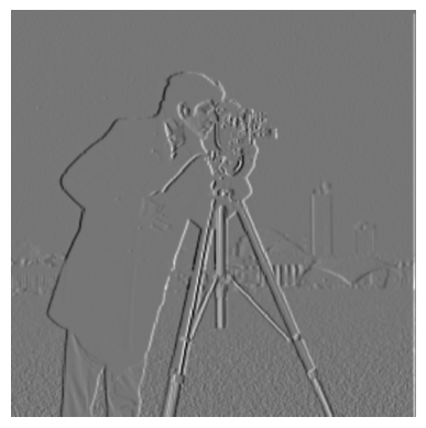
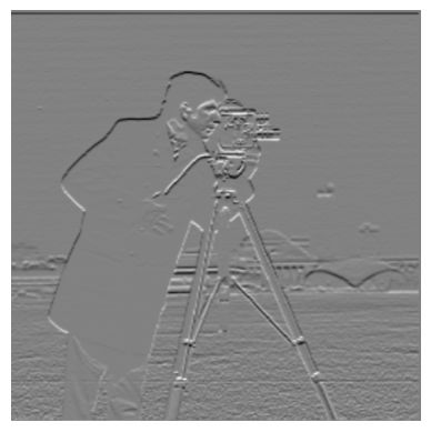
First, we will use a simple finite difference operator applied in the x and y direction.
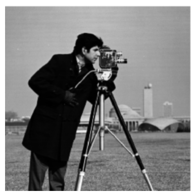
As we learned in class, this approximates a partial derivative in the x and y direction, and large values represent a sudden change in pixel values - likely some type of edge. We can use these operators applied as a convolution onto this greyscale image of a cameraman.
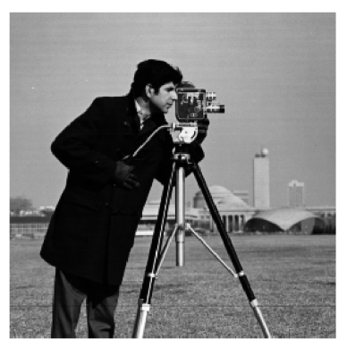
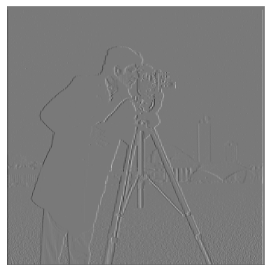
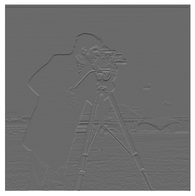
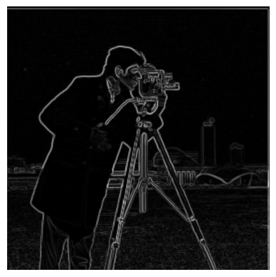
We can improve upon this by combining the derivatives in the x and y directions using a simple L2 formula, providing a better view of the edges of the images. After that, we can easily binarize it by trying out a range of thresholds. Noise that is below this threshold will be eliminated, while values at or above the threshold will be set to 1 to show that we’ve found an edge. The computation for the magnitude is simply:
\[M = \sqrt{D_x^2 + D_y^2}\]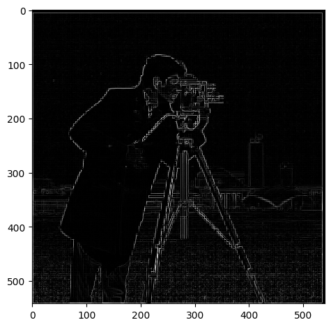
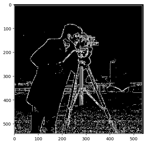
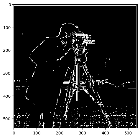
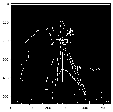
As one can see here, a lower threshold is ineffective at removing noise (such as the grass at the bottom half of the image) while the higher thresholds contained more junk data. Threshold=0.15 strikes a decent balance, keeping important edges and details in the background (such as the tower) while keeping just a bit of grass at the bottom of the image. It’s also interesting to note that edges in the background, which appear more gray, tended to have smaller magnitudes simply because the color values aren’t as strong as the foreground - showing a fundamental flaw in our operator with its lack of normalization.
Task 1.2: Derivative of Gaussian Filter
Even with a decent threshold though, we can see that there is a lot of noise with our difference operator. By first applying a smoothing operator, we can remove much of the noise. Here, we’ll create a Gaussian filter to essentially blur the image and repeat the process above, yielding the following image and the corresponding magnitude:
As with before we can binarize this and use a range of thresholds to see which works the best.
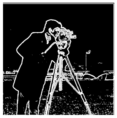
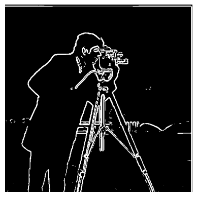
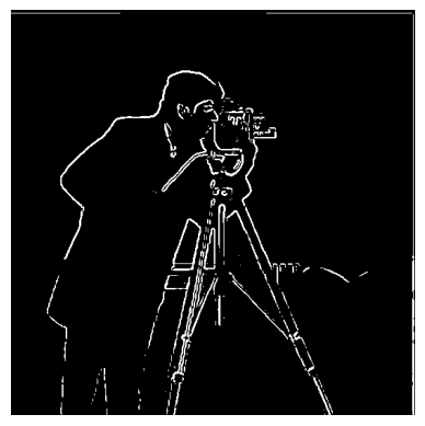
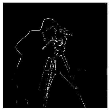
As we can see here, a threshold of 0.12 pretty much removed all noise from the image and was able to preserve many of the edges within the image. The difference between this edge image from our attempt previously is that it’s much smoother - rather than “blocky” straight lines and lots of little dots caused by noise we have continuous looking lines that much better match the contours of the cameraman’s body. The smoothing filter essentially smoothed out the detected edges and gave us a much better result than before.
Combining Convolutions
In order to make this operation even faster, we can actually combine the 2 separate convolutions - blurring and then the difference operators - into one before applying it to the image.
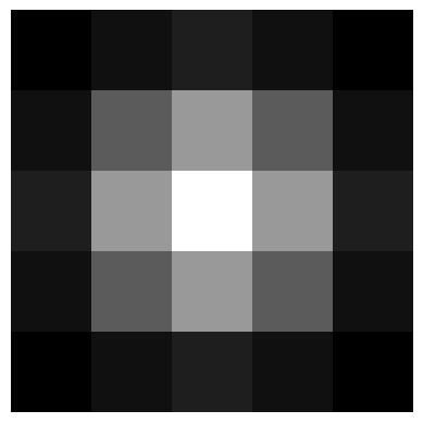
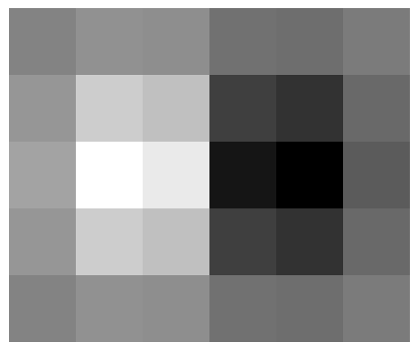
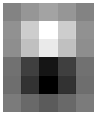
Comparison of Combined vs Seperate Convolutions
The resulting partial derivative of Gaussians (DoG) were the same, and putting it through our L2 operator and using the same threshold ended up with the exact same result - except that combining the convolutions together made the operation way faster!
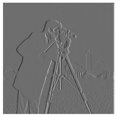
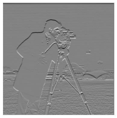


As expected, we get the same results!
Task 2.1: Image “Sharpening”
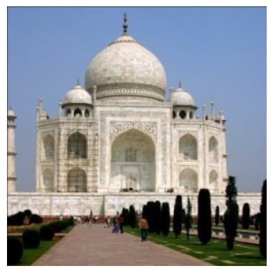
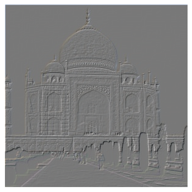
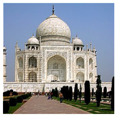
After blurring images, we can try to “unblur” them by “sharpening” them, essentially making the high frequency data (mostly the edges) appear stronger within an image. To do this, we want to essentially do the opposite of the blur filter:
- Blur the image with a gaussian filter.
- Take the original image and subtract it by the blurred image. This leaves the high frequency details
- Multiply these high frequencies by a muliplier alpha. Add it back to the original image to get our sharpened image.
As with before, we can actually combine these operations into one. To “invert” our low-pass filter (Gaussian filter), we can use a impulse unit filter (matrix the same size as the gaussian filter with 0s everywhere except the center) and subtract it by the low-pass filter. This essentially gives us a high-pass filter. We then arrive at a simple formula:
\[(1 + a) * inverse\_low\_filter + low\_pass\_filter\]That will provide us a single convolution that sharpens an image. The result and its intermediary results are shown below.
Sharpening the Taj

Blurry Cat
Let’s try this out on another blurry image with varying alpha - say this blurry picture of a cat.
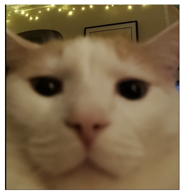
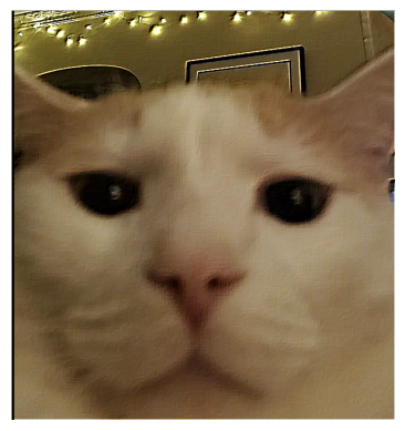
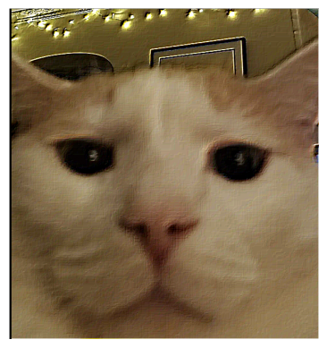
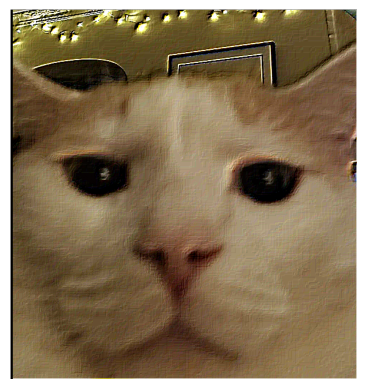
As we can see, the sharpening does appear to make the image less blurry, and as we increase the alpha, the edges get more pronounced. At a certain point though, a higher alpha just makes the edges way too strong - such as in the case of a=20 the lights in the background start looking quite unnatural.
But what happens if we try to take a decent picture, blur, and then sharpen it again? Let’s try that on a picture of the Campanile.
Blur, Then Sharpen, The Campanile
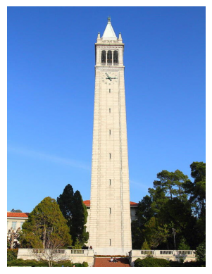

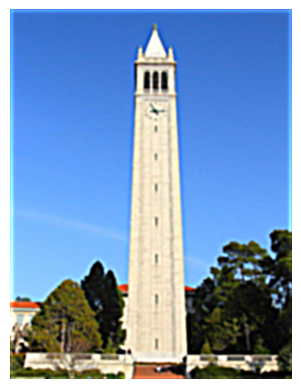
As we can see here, the sharpened image unfortunately doesn’t look exactly like the original image. Although the edges are sharpened and more discernable than the blurred image, there are elements of the image that sharpening simply can’t recover after being blurred.
Task 2.2: Hybrid Images
Using the SIGGRAPH 2006 paper by Oliva, Torralba, and Schyns, we can use what we’ve done above to create Hybrid Images! The idea is simple - the human eye works such that at close distances we mostly notice the high frequency details, while far away we notice low frequencies more. Therefore, by taking 2 images and combining the high frequencies of one and the low frequencies of another, we can create hybrid images that look different when seen close vs far away.
We’ll first use the class example - Derek and his cat Nutmeg. We’ll take the low frequencies of Derek and the high frequencies of Nutmeg, align the images, and combine them to create CatMan.
Cat Man Hybrid

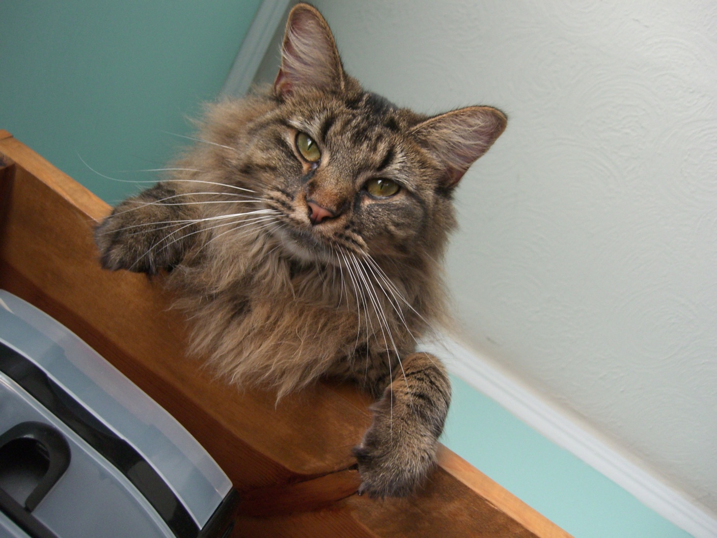

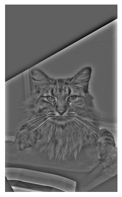
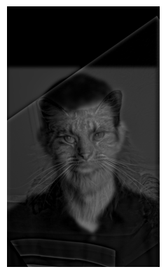
If you look closely, cat man appears to be a cat (albeit with faint traces of a man in the background). Zoom out or walk away from the screen though and the cat fades away to reveal Derek.
Let’s try some other examples.
Hybrid #1: Campanile/Hoover Tower Hybrid

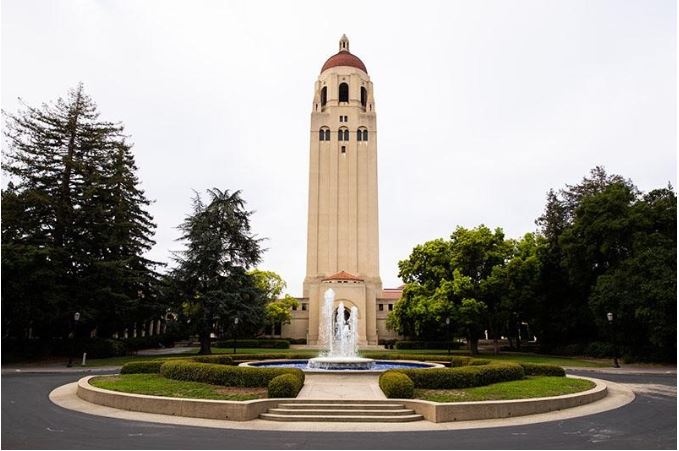
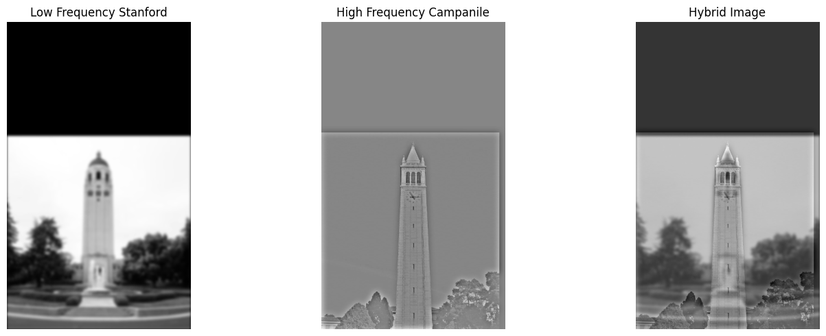
Legend has it that Stanford asked Berkeley for the campanile’s height when creating their clock tower, only for Berkeley to lie and give them the wrong measurements so that they create a shorter tower than ours. Inspired by that, here’s a hybrid of two of their most prominent towers. Funnily enough - from this angle it does appear that Stanford’s Hover Tower is shorter.
Hybrid #2: The PTSD of CS162 (Failed)
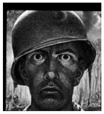
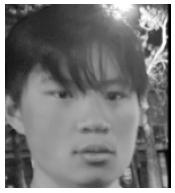
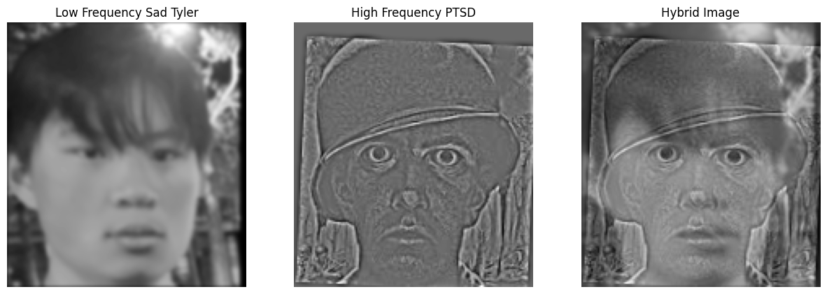
Here we have a hybrid image that didn’t work as well. In this picture, I wanted to merge Tyler, my 162 teammate, with the classic art of a soldier experiencing PTSD, to show the visual similarities between a person who endured 162 and a soldier of war. Unfortunately, no matter how far away you look the black pits of the PTSD soldier’s eyes are pretty hard to ignore, overshadowing the lifelessness of Tyler’s eyes. This shows that color is also an important aspect with the hybrid images - solid blocks of pure black (such as in the PTSD soldier’s eyes here) aren’t as affected by the filters, and are prone to sticking out. There’s also the issue that the PTSD soldier’s art was in general a darker hue than Tyler’s picture due to lighting. Perhaps normalization between the two images could’ve helped with this… or maybe that’s just a fundamental difference between the difficulty of going to war vs taking CS162.
Hybrid #3: Hybrid Hank
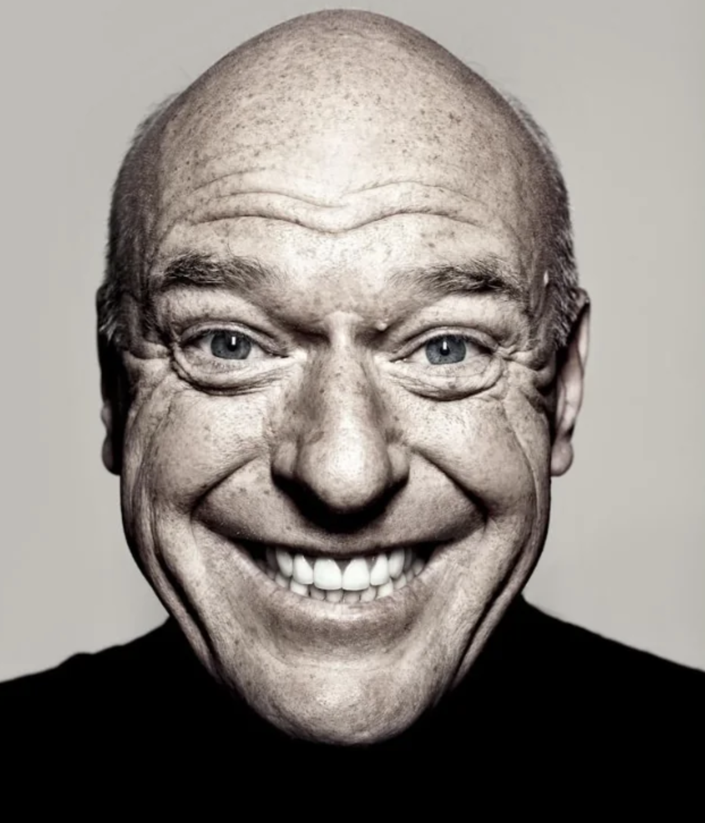
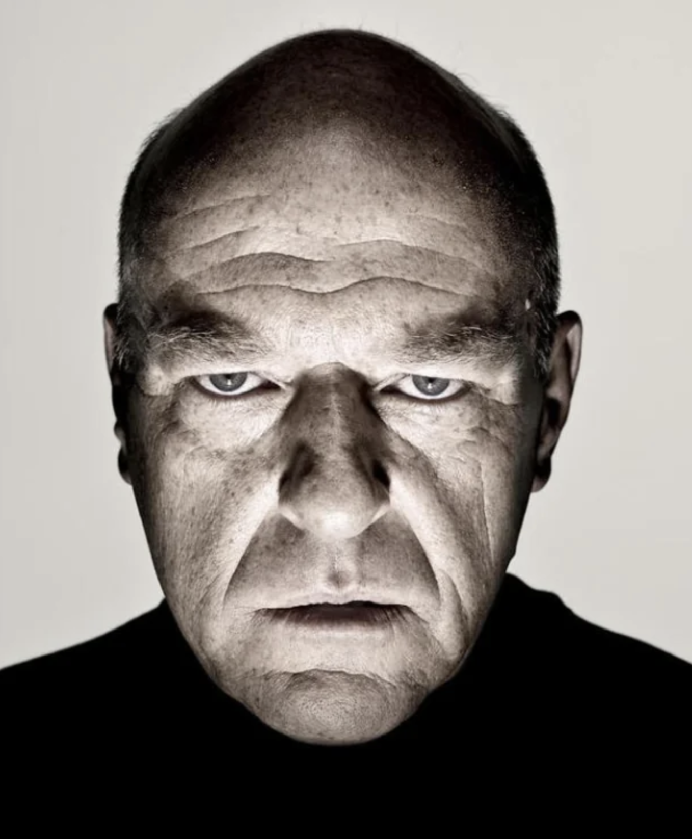
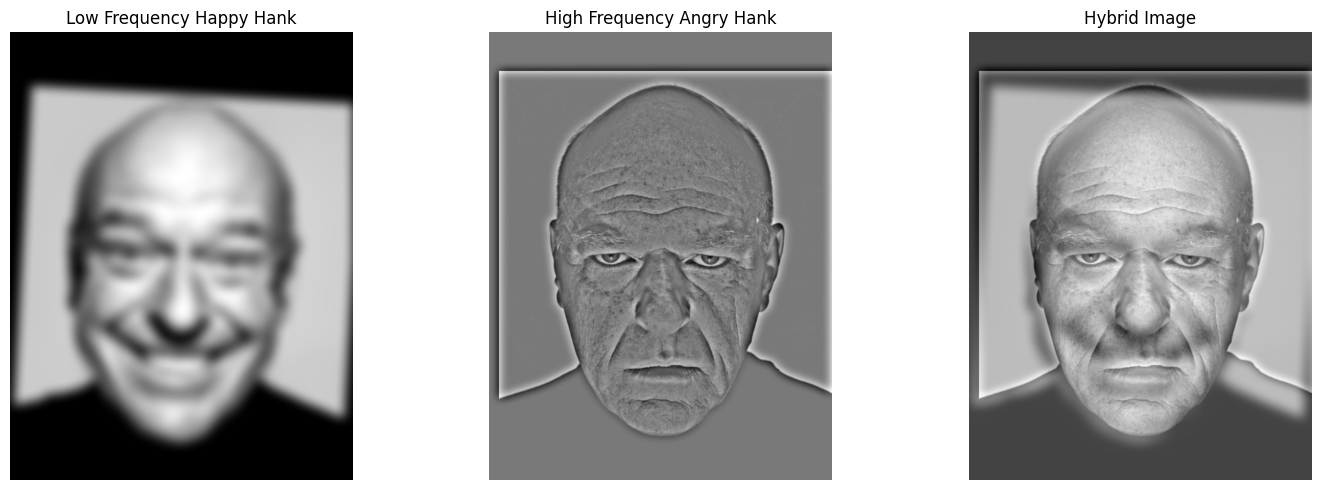
Here we have my favorite: a merge showing a change of expression for Hank, from the hit show Breaking Bad. Far away, Hank looks relaxed and happy. Upon closer inspection however, he reveals himself to be deeply suspicious and angry about something. The in the expressions made this a popular meme format online, and it was very fun making it into a hybrid image.
We can also use FFT to see what were the effects of applying a low and high pass filter to these images, so that we can better understand how it created this hybrid image
Hybrid Hank FFT Analaysis
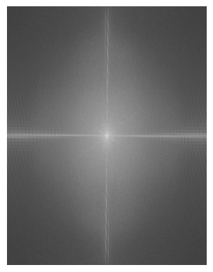
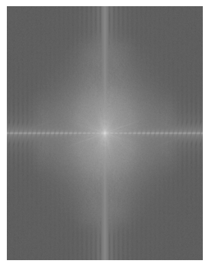
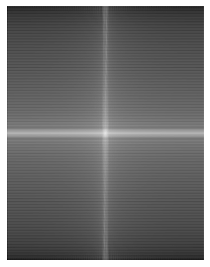
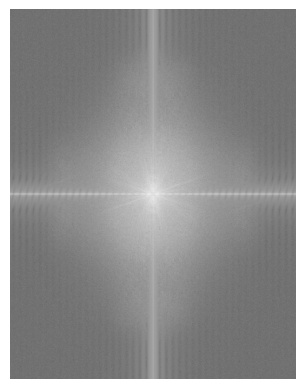
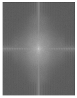
We can clearly see that, as a result of the low-pass filter, the Fourier transform of Happy Hank has much of the high frequency details removed - all that’s left are low-frequency details as represented by the white horizontal and vertical lines. For Angry Hank, the high-frequency details are way more prevalent. This image was probably successful due to the greyscale nature of the image and the highly compatible nature of the two images - they are literally aligned already and have the same overall structure.
Task 2.3: Gaussian and Laplacian Stacks
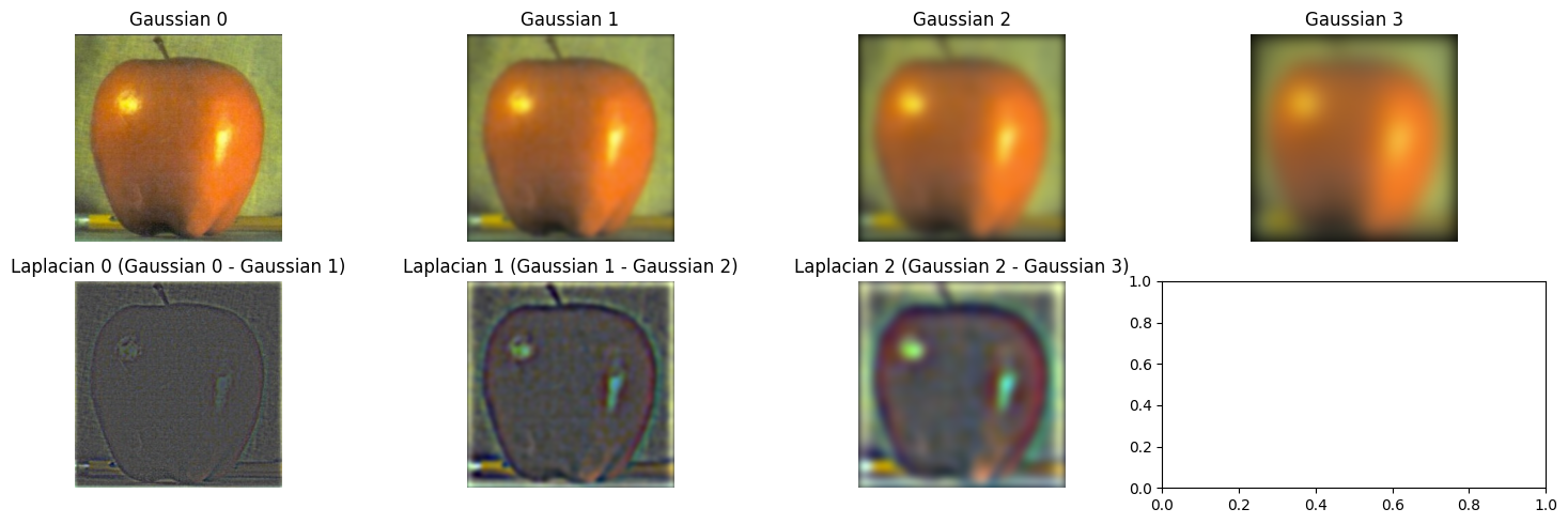
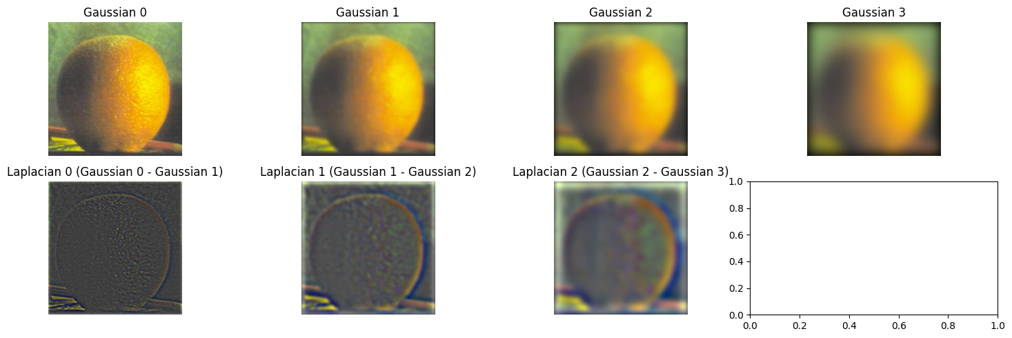
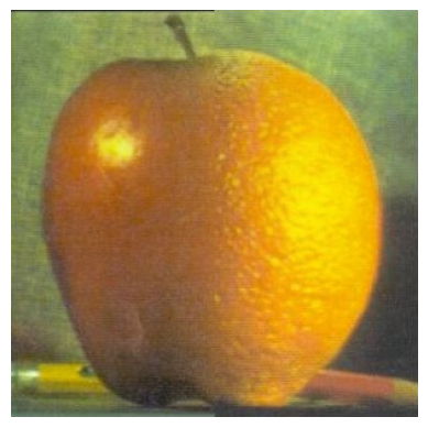
What if we applied the gaussian filter to a image multiple times? Then we get a Gaussian stack, and by subtracting between successive levels of a gaussian stack we get the Laplacian stack instead. Here’s an example with the Orple.

The interesting thing here is that by taking the blurriest image in the Gaussian stack and adding it to all the images from the Laplacian Stack, we can get back our original image. This is because each image in the laplacian stack stores the lost information between each successive application of the Gaussian filter.
Task 2.4: Multiresolution Blending
With the Laplacian and Gaussian stacks, we can now do multiresolution blending, (nearly) seamlessly combining two images. To do so, we follow this algorithm:
- Create a Gaussian and Laplacian Stack from the two images you’d like to merge
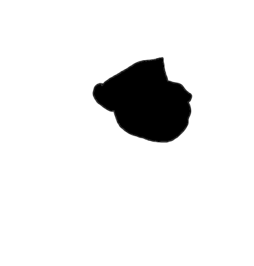
- Create a mask, with 1s on one half and 0s on the other. The dimensions of the two images and mask must be the same.
- Create a Gaussian stack from the mask. Let N be the number of levels in all three of these stacks.
- Multiply Image1_Gaussian[N-1] with Mask_Gaussian[N-1], and Image2_Gaussian[N-1] with (1 - Mask_Gaussian[N-1]).
- For levels 0 - N-2, multiply Image1’s laplacian with the corresponding mask, and Image2’s laplacian with the corresponding (1-mask).
- Add all the resulting images from 4-5 together.
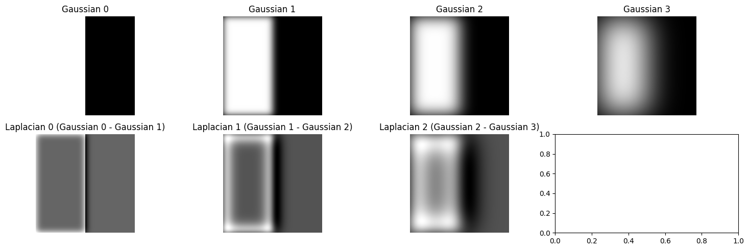
As stated before, the blurriest image + the Laplacian stack perfectly recreates the original image. The mask acts as a weight to determine how much a particular pixel on the resultant image should be affected by either image. By applying a Gaussian filter onto the mask, we essentially blur it, and when we apply the different blurred masks to the Laplacian stacks of each image, we get a much more seamless blend of the two images, while still perfectly preserving the details of either image.
Orple Blending Process
Blending Example 2: Cat Loaf
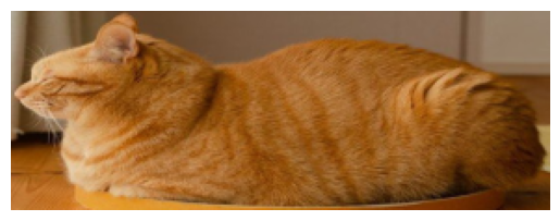
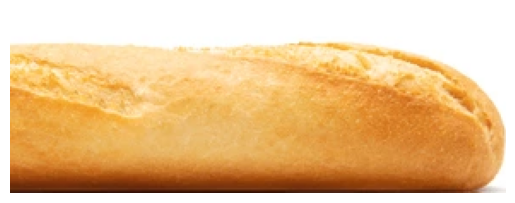
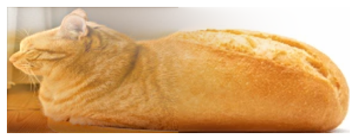
Next, I tried to use this technology to figure out why cats sitting with their paws tucked in are referred to as “loafing”
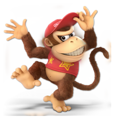
Blending Example 3: Hybrid Kong
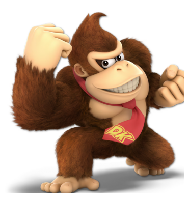
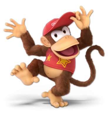
For our last example, let’s try cropping out a face and putting it on something else - here I’ve chosen Diddy and Donkey Kong’s portraits from Super Smash Bros.
