CS180 Project 3
Face Morphing and Modelling a Photo Collection
Task 1: Establishing Correspondences
Before we get to the main event of Face Morphing, we must establish keypoints in the two images we’d like to morph. The important thing here is that:
- The images have the same size
- Each point pair in the images must be associated with each other
- Optimally, glasses and other accessories are taken off.
- Use a good number of keypoints and place them in good spots (optional)
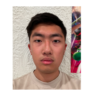
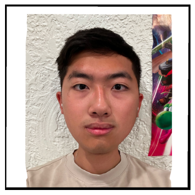
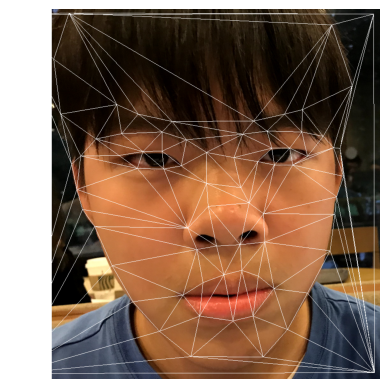
To troll my high school friend Andrew I decided I want to make a face morph between him and me. The following are the points I created using the tool provided on the CS180 website
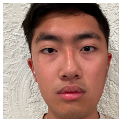
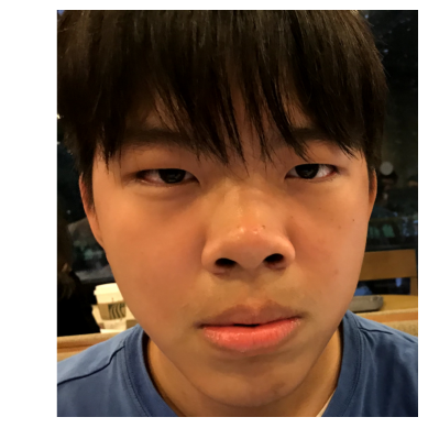
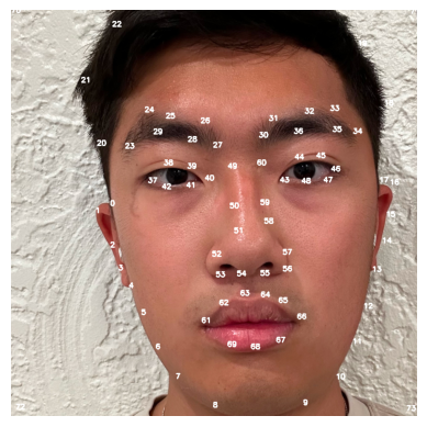
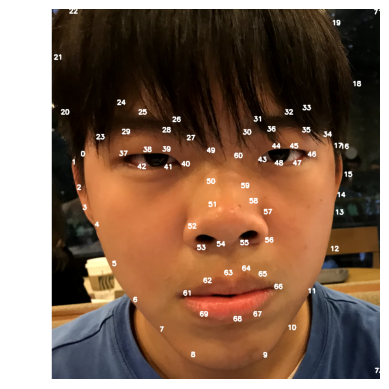
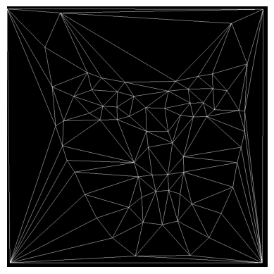
By using a Delauney Triangulation, we generate a very good triangular mask of the images. This will help us morph the faces later. Each triangle in our source image (Me) corresponds to a triangle in our destination image (Andrew), and our goal will be to shift the pixels such that we can blend one triangle’s details with the other’s

Task 2: Getting the Average Face
With our triangulations from Part 1, we can now calculate the “average” face between me and Andrew. The overall process looks like this:
- Find the average mask between the two images first. For each pair of points, find their midway point and apply the same triangulation to all 3 image points (Me, Andrew, and Midway)
- For each triangle t in source image (me), and corresponding triangle t’ in average mask:
- Compute the affine transformation from t to t’. More information below.
- Compute the inverse of the affine transformation from (1).
- Apply the inverse affine transformation to all points in the destination triangle. Now, each point will be transformed to a mapped coordinate in the source triangle, which represents the pixel value the destination pixel should take.
- Use some sort of interpolation method (or nearest neighbor/round) to get the source pixel value from the mapped, and apply it to the destination pixel.
- Repeat for each triangle t in the destination image, and average the pixel values taken between the two source images.
To get the Affine transformation, we can use the handy formula that was on Edstem:
\[\begin{bmatrix} p_{x_1} & p_{y_1} & 1 & 0 & 0 & 0 \\ 0 & 0 & 0 & p_{x_1} & p_{y_1} & 1 \\ p_{x_2} & p_{y_2} & 1 & 0 & 0 & 0 \\ 0 & 0 & 0 & p_{x_2} & p_{y_2} & 1 \\ p_{x_3} & p_{y_3} & 1 & 0 & 0 & 0 \\ 0 & 0 & 0 & p_{x_3} & p_{y_3} & 1 \end{bmatrix} \begin{bmatrix} a \\ b \\ c \\ d \\ e \\ f \end{bmatrix} = \begin{bmatrix} q_{x_1} \\ q_{y_1} \\ q_{x_2} \\ q_{y_2} \\ q_{x_3} \\ q_{y_3} \end{bmatrix}\]solving for a, b, c, d, e, f allows us to create an affine transformation such that:
\[\begin{bmatrix} a & b & c \\ d & e & f \\ 0 & 0 & 1 \end{bmatrix} \begin{bmatrix} p_{x_i} \\ p_{y_i} \\ 1 \end{bmatrix} = \begin{bmatrix} q_{x_i} \\ q_{y_i} \\ 1 \end{bmatrix}\]where p is our source point, and q is our destination point.


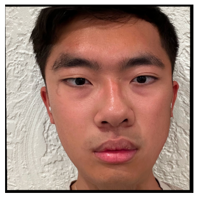
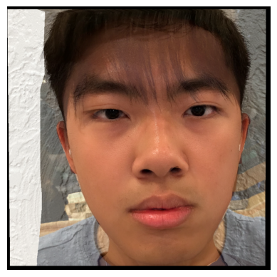
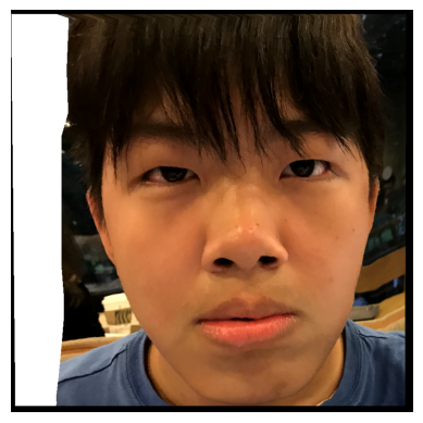
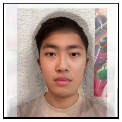
The result was better than expected, as I was worried the differing hairstyles would get in the way. Although it’s still weird to see transparent hair, everything else looked pretty good. It disturbed a couple of my high school friends and Andrew himself since both our distinctive features are there, so mission accomplished.
Task 3: The Morph Sequence
By playing around with our method from before, we can introduce a warp_frac, and dissolve_frac value.
Rather than always computing the midway face by averaging the points/pixels, we can use the values to adjust how much warping we want as well as how much cross-dissolving the pixels should do. For face warping, we’ll simply use the formula
\[point_{new} = point_{src} + (dest_{src} - point_{src}) * frac_{warp}\]and rather than applying 50% of each source image’s pixel values, we’ll use dissolve_frac for the source image, and 1-dissolve_frac for the destination image.
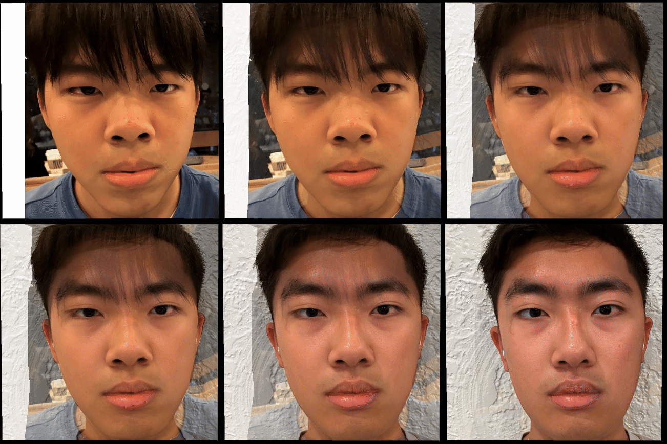
If we then slowly increase these values from 0 to 1, we get a smooth warp sequence detailing how the face changes:
Part 4: The “Mean Face” of a Population
But what if we applied this to multiple people? By taking many well-aligned pictures of different people, we can use our morph function to find the “mean face” of a population. The process goes as follows:
- Find the “midway mask” amongst all the faces and their points. Simply average across the x and y values for a point.
- Warp each face into the new midway mask using the morph method we created above
- Overlay each face onto one another and divide by the population size to get the mean face.
I used the Dane dataset. Here are some examples of points, the midway mask, and how people looked after morphing the points to the midway mask.
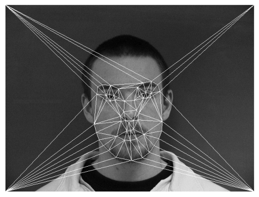
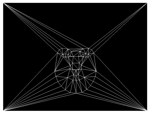
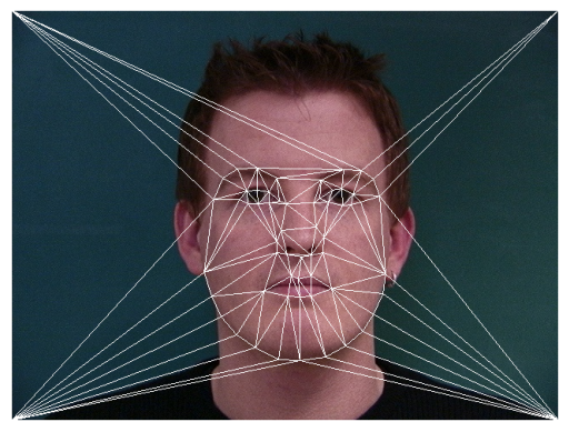
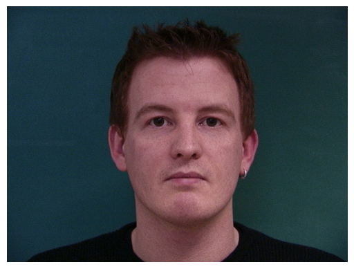

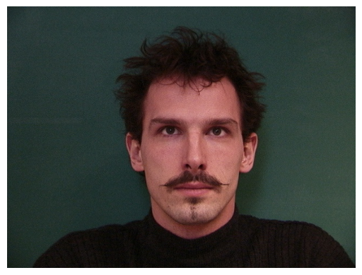
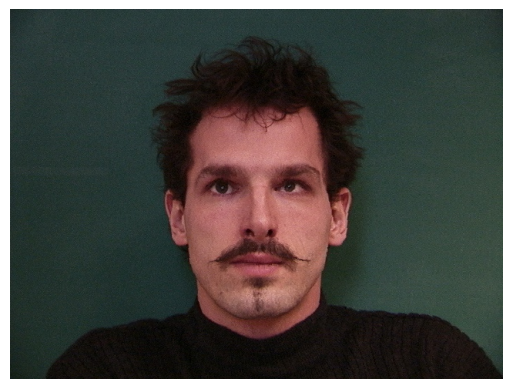
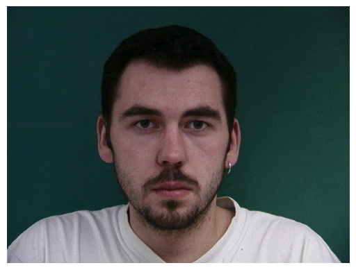
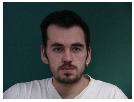
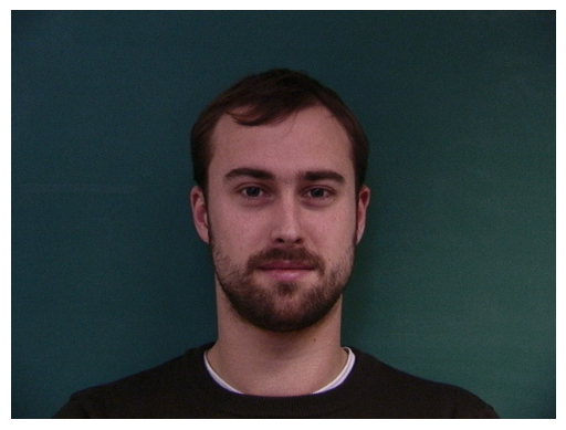
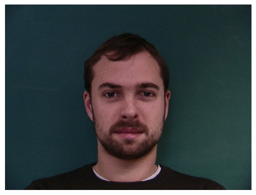
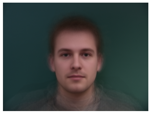
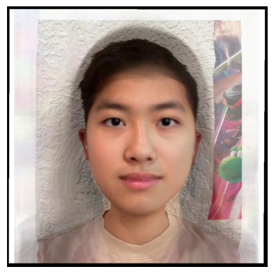
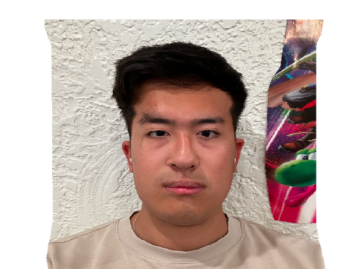
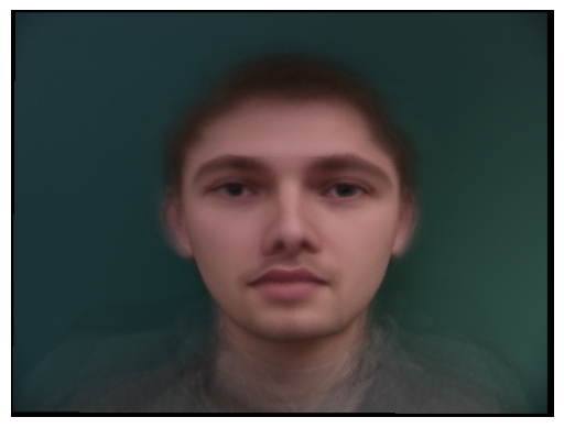
We can even have some fun with this, morphing the dane face to my face, or morphing my face to the shape of the average dane’s face to simulate an idea of how I might look as a Dane.
Part 5: Caricatures
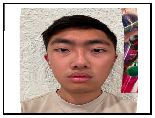
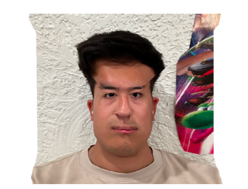
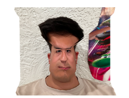
Unfortunately the Dane face warping didn’t come out too good, but there are ways we can adjust that. As with warp_frac before, we can introduce a multiplier to determine just how much I’d like to warp my face to a destination mask. If I specify 1, it’d be the exact same result as what we saw just now. Lower values would mean I’d get lesser amounts of the differences between the average Dane’s features and mine, reducing the weird warping we see in the previous image. If I use a value above 1, I create a caricature - where I actually gain too much of the Danes’ features.

Bell and Whistle: Changing Genders
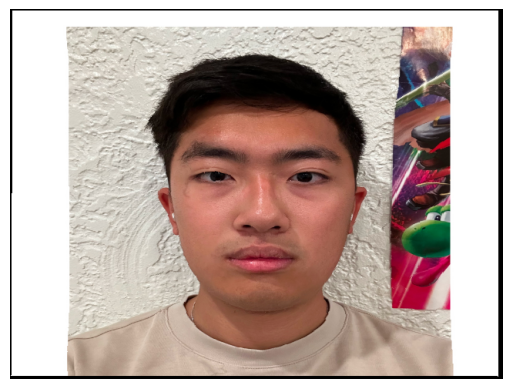
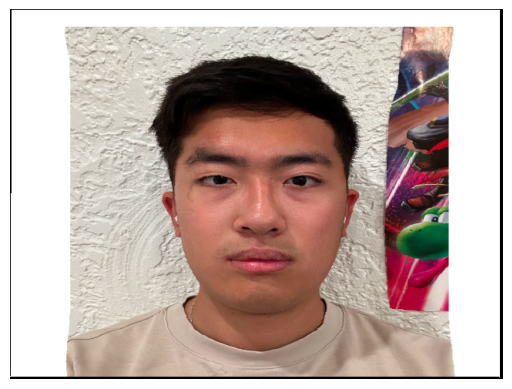
I found an image of the average female face for Hong Kong women attending a specific university, which was the perfect way for me to test how I might look if I was female considering I’m from Hong Kong myself, plus the age range of the faces were appropriate as well. After adjusting some of the multipliers, here were the best results I got, with just warping the face shape, the appearance, and both.
