CS180 Project 4
Image Warp + Mosaic
Task 1: Taking Pictures (Rectification)
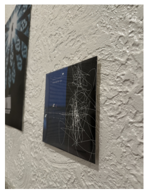
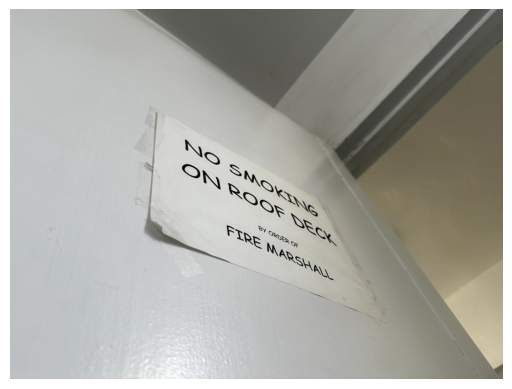
Our first task is to take a couple of pictures of rectangle-shaped objects from different angles, and try to rectify them. I chose 3 different pictures below: a vinyl cd, a no-smoking sign, and finally a rectangular window. I’m particularly interested in the window as the effect of rectifying gives the illusion that we’re standing right in front of the object thus making it rectangular, but we obviously can’t see straight out the window as our view is from the side, so what would the effect look like in the finished image?

Task 2: Recover Homographies
Next, we need to recover a homography to transform the images. In our first problem of rectification, the idea is simple: Label the 4 corners of the images, select 4 additional points to create a rectangle (roughly the same shape as the original object), and recover a homography from the image’s 4 corners to the rectangle.
Here are the pairs of points that were chosen for the images:

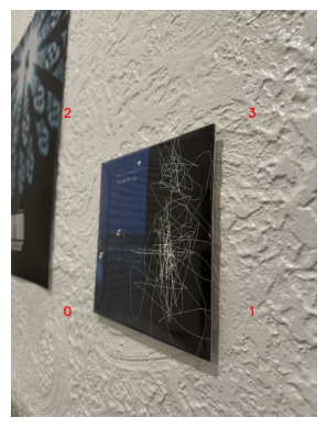
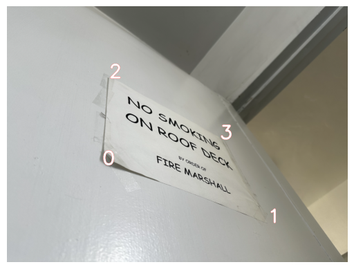
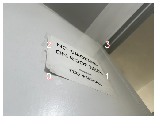

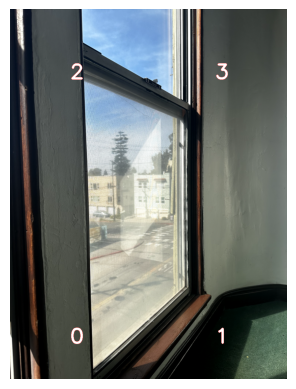
After setting the points, we set up the equation p’=Hp, where p’ is our destination points and p is our source points, and solve for H. In this case, since we have 4 points, there is only one possible H that can satisfy the equation. For mosaics though, we’ll choose more points for stability, so we’ll make an overdetermined system and use least squares (or SVD) in order to find the best solution.
To solve for H, we’ll use the equation we learned in lecture, and use SVD to find the least squares solution:
\[A = \begin{bmatrix} x_1 & y_1 & 1 & 0 & 0 & 0 & -x_2 x_1 & -x_2 y_1 & -x_2 \\ 0 & 0 & 0 & x_1 & y_1 & 1 & -y_2 x_1 & -y_2 y_1 & -y_2 \end{bmatrix}\]By then using SVD, decomposing the matrix into the form:
\[A = U S V^T\]The least squares solution will be in \(V^T\), which has 9 variables
We reshape this into a 3x3 matrix, and then by dividing the entire matrix by the last variable (I), we get an H of the form
\[H = \begin{bmatrix} h_1 & h_2 & h_3 \\ h_4 & h_5 & h_6 \\ h_7 & h_8 & 1 \end{bmatrix}\]Now, if we plug in a particular point (with a one appended to it) from the image, the resulting point will look like:
\[\begin{bmatrix} wx_2 \\ wy_2 \\ w \end{bmatrix} = H \begin{bmatrix} x_1 \\ y_1 \\ 1 \end{bmatrix}\]Dividing the resulting point by w yields \(x_2\) and \(y_2\), giving our new coordinates.
Task 3: Warping the image (Image Rectification)
Now that we have the homography, it seems trivial to simply pipe each point of the original image through the homography to get the new coordinates of that pixel, giving us our result. However, this is forward warping, and as we’ve seen in project 3 this results in tons of holes. Therefore, we need to use inverse warping instead. Thus, the algorithm looks very similar with our triangle warping function from Project 3:
- Find the homography H from src_points to dst_points
- Take the inverse, yielding H’
- Determine the dimensions of the resulting image by warping the 4 corners of the src image through H. Shift the entire image if there are any negative values so that the negative values become 0.
- For each point in the resulting image, apply H’ and interpolate to find the src image’s corresponding pixel value, and apply it.
We can also vectorize 4 by making a 2D matrix of all the points in our result image, yielding a way faster result. We’ll ignore any points that are outside of the convex hull of the warped bounding box.

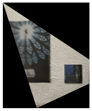

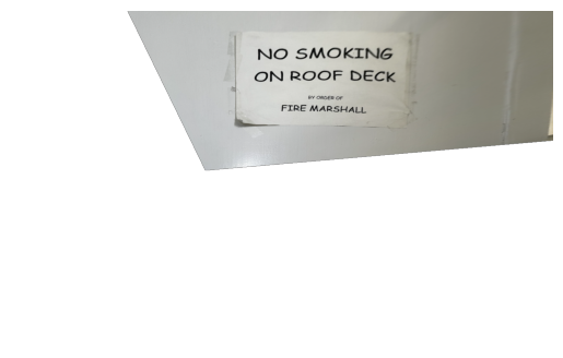

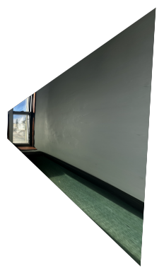
The results surprised me, giving us the illusion that we’re looking at the images from a new point of view. The window one shocked me the most. We weren’t able to see more of the scenery outside of the window (of course), but a shift in the perspective and perceived distance from the window warped the window to a rectangular shape.
Task 4: Image Stitching (Manual)
Lastly, we come to image stitching. At a high level the steps are to:
- Take a pair of images with significant overlap. Label common features/points between the two images
- Create a homography to map the second image’s points to the corresponding points in the first image
- Warp the second image using what we created in Task 3
- Align the images together, and blend.
First, let’s take a couple of pictures:


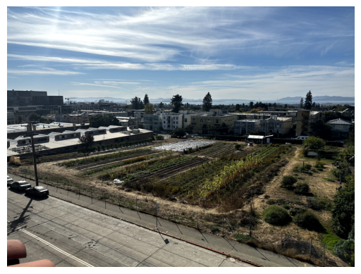

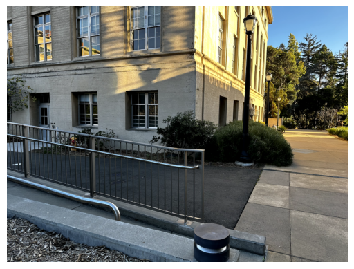
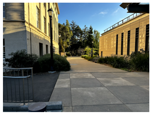
Next, let’s label some correspondences between them manually.
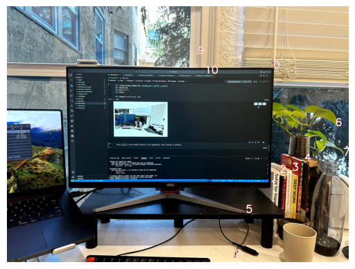
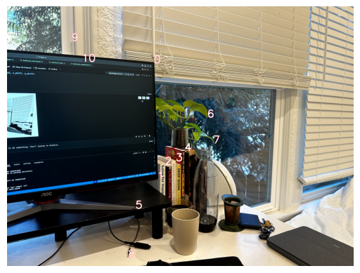
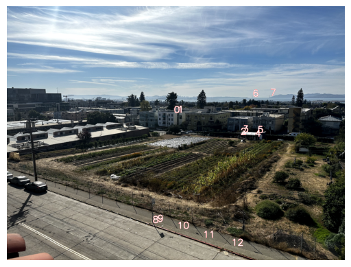
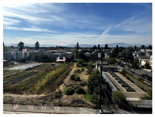


Then, we warp the second image using the homography recovered

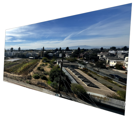

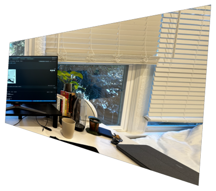

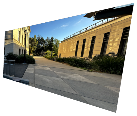
Now, we need to align. Unfortunately if we stacked one image atop the other, the borders will be really obvious. Therefore, we need some form of blending. The algorithm I came up with is:
- Recover x_shift and y_shift from inverse warping. We found this when applied H to the bounding box of image 2 while inverse warping.
- Reshape image 1 so that the height of the image is the same as image 2, and apply y_shift so that they are aligned in the y_axis.
- Apply x_shift to image 2 so that the x_axis is aligned.
- Find the overlapping image (all points with x value between x_shift and im1.width)
- Fill in the non-overlapping areas with image 1 on the left and image 2 on the right.
- In the overlapping area, use an alpha value that begins at 0 at the left side and increases to 1 on the right side. Use a weighted sum of image 1 and image 2, multiplying image 1’s pixel values by (1 - alpha) and image 2’s by alpha.
This results in the following images:
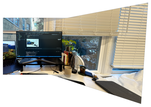
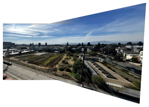
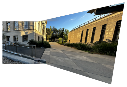
One issue is the strange triangular gray areas in the overlapping region. We can fix this by using a for loop to detect points in the overlapping region where one image is out of bounds. If that’s the case, use only the pixel values from the image that isn’t out of bounds.
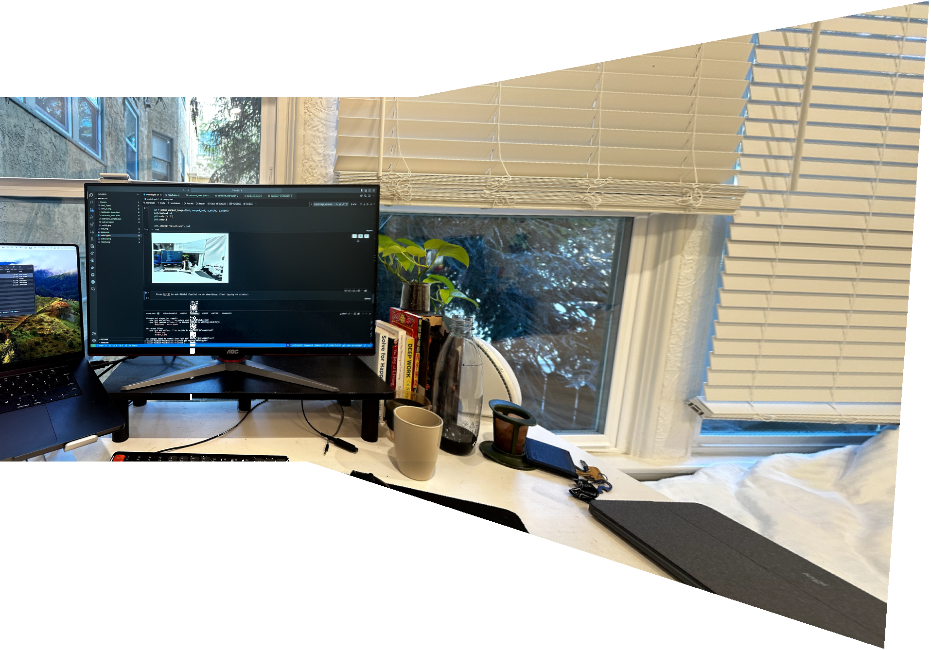
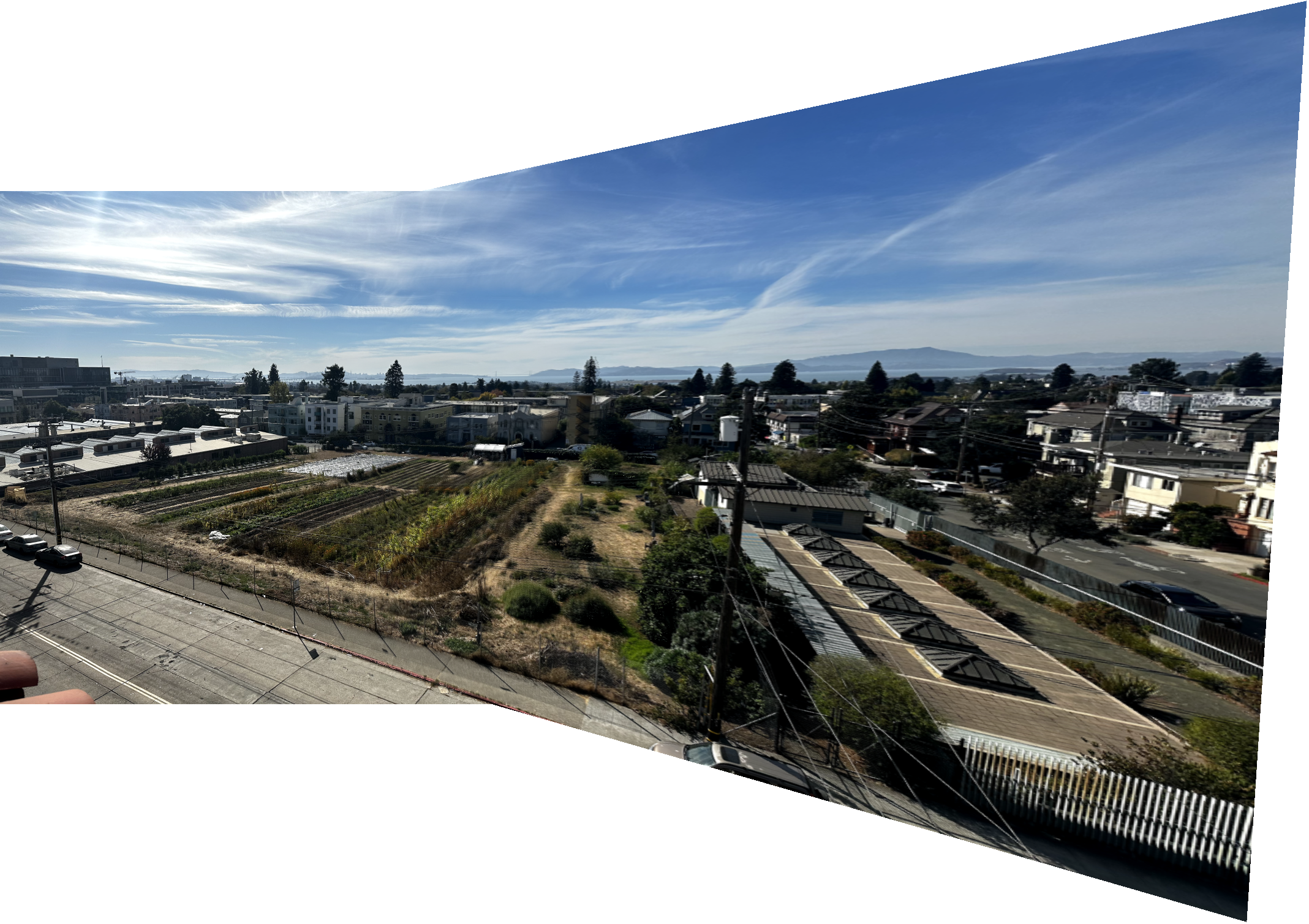
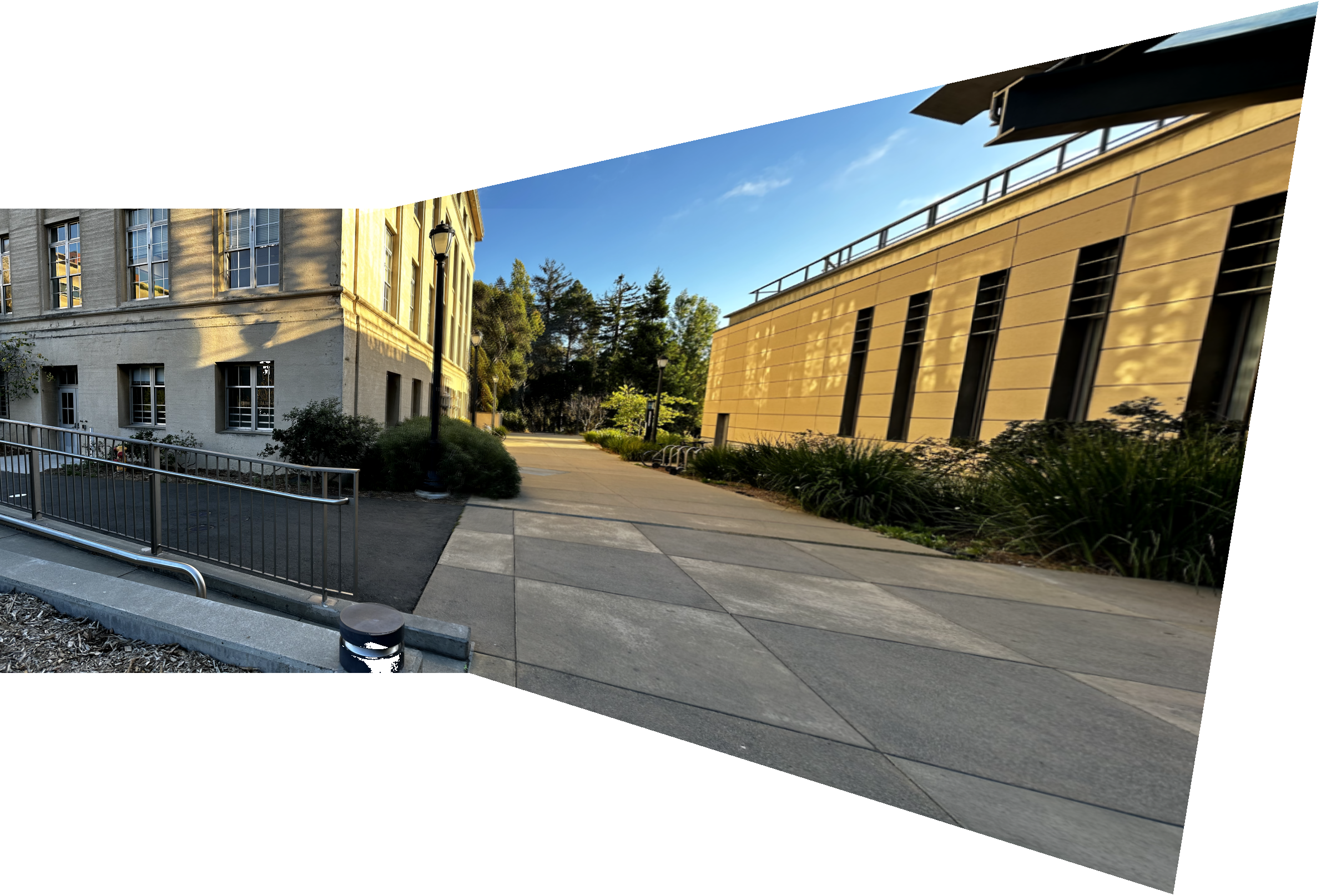
Overall, this project was immensely satisfying and it was fun taking some of the functions and logic that was written in project 3 and reusing it. As a kid I always thought it’ll be easy to make panoramic shots - just blend many images together! But this project proved otherwise, and showed that there are many optimizations and changes needed before it looks decent.
Another key learning from this was the importance of good labeling. I tried only using 4-5 points for the balcony picture and that resulted in disaster, where the roads were obviously not lined up. I realized it’s because I was mostly using features at the top of the image and neglected points at the bottom. I was surprised that adding twice the number of points and adding more points at the bottom of the image made the stitching far far better.
Task 5: Image Stitching (Automatic)
Onto the fun part: Stitching the images automatically!
In theory, the idea is straightforward. All we need to do the stitching above are correspondences between our two images, and as similar parts of the image would necessarily have similar pixel values, if we can find a way to smartly find features between the two images and match them, we can automatically stitch it into a mosaic.
Thus, our first step is to find good points in both images that we can match - in particular, we can use the given Harris Corner detectors, which uses a combination of the vertical and horizontal derivatives (similar to project 2) to find areas where both derivatives are high - which tend to be corners in the image.
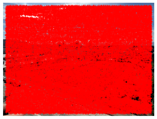
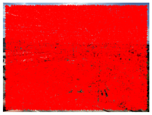
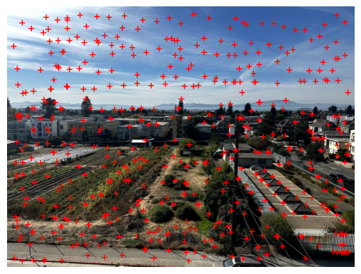
There’s a clear problem here: There’s way too many! Luckily, each harris corner has a harris strength we can use to filter out points that are more likely to be corners vs those that are not.
It may seem natural then to just select the k highest strength harris corners, but that would lead to clumps of harris corners, when we’d like an even spread of strong corners in most parts of the image. Therefore, we’ll use Adaptive Non-Maximal Suppression.
The idea of ANMS is that each strong corner will have a “radius” of suppression that will ignore all other corners within that radius. We iterate through every Harris corner and calculate what the maximum radius that will be for each point without suppressing a significantly stronger corner - giving us the “best” radius a corner can have without ignoring an even better corner.
We then simply take the k harris with the highest “best radius” - these would be points that are strong in their local region. This way, we get a much better spread of harris corners throughout the image, while still keeping the strong corners and ignoring weak ones. As we saw in task 4, it’s super important to have a good spread of correspondences, so this step is crucial!
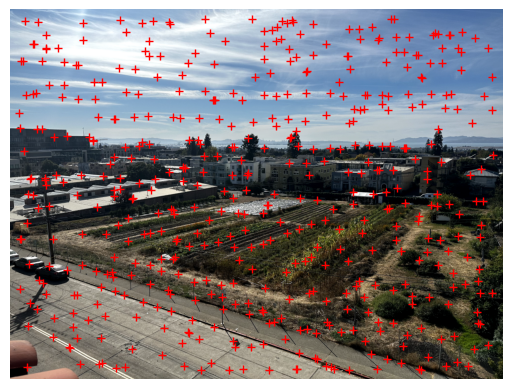
Now, we need to match Harris corners to each other. To do this, we need to take the Harris corner point and get the local features. For this, we’ll take a radius=20 area around the point (a 40x40 square) and use a step of 5 to yield a 8x8 descriptor. We can then further bias-gain normalize it to ensure it has a mean of 0 and std of 1 across each channel. This is a simplified version of the “Multi-Scale Oriented Patch” we went through in lecture, and works very well in matching points with each other.
By using these corners and computing the pairwise L2 distance between all pairs of corners between the two images, we can gauge just how likely two harris corners correspond to each other.
Below is an example of a descriptors from the image above, at the dot on the left image.
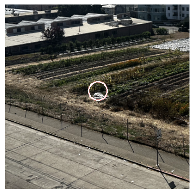
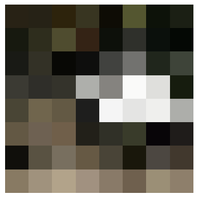
Looking at the image though, there are some points that just don’t seem like they’ll pair well. Like the ones in the sky for the example above - those would give a feature that’s mostly blue, so how would that give a good match?
To deal with this problem, we’ll be smart with the way we match local features. For each local feature, we’ll find the 2 nearest neighbors in terms of L2 distance. We then calculate the ratio of the best match’s distance divided by the second-best match’s distance. If the match is unique, this ratio should be very low. We’ll set a threshold and ignore any ratios that are higher than that. This yields the following result and matches:
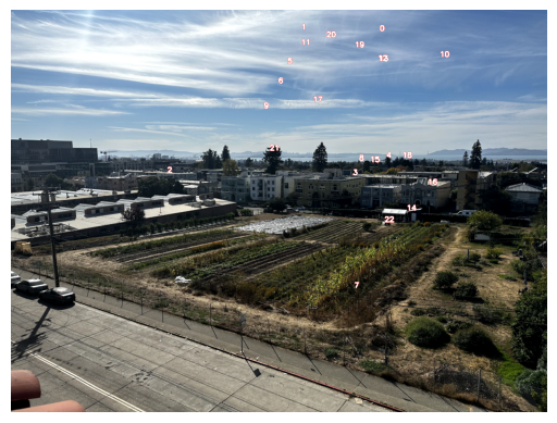

(From my own testing, it appeared threshold=0.4 was best, but here I chose 0.5 to show the effects of RANSAC later.)
Regardless, it looks like we got some pretty good matches! There’s just one obviously wrong choice - the “2” match we can see towards the left of the image. Thus, we’ll use the next part - RANSAC - to find a good homography.
Since some points may still be outliers (like 2 here), we can utilize Random Sample Consensus to find the best point matchings for calculating the homography. As described in lecture, the algorithm goes:
- Select 4 random correspondences and find the homography matrix.
- For all points, generate a list of “inliers” by feeding each image 1 point through the homography
- Calculate the distance between the result and the real image 2 point that it corresponds to. If it’s below some threshold e (I used 1), it’s an inlier.
- Keep track of the biggest list of inliers
- Repeat 1-4 a maximum of n times.
- Use the best list of inliers as correspondences for computing the homography.
In the end, this was our best list of inliers:

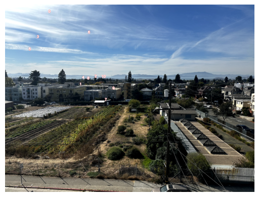
To my dismay there were no good points towards the bottom of the image, but hopefully that won’t cause too many issues in the future.
Next, we just have to treat this like our images from 4a and mosaic them. This is the result, shown alongside the manual result to compare.


Amazingly the results were both very very close, although the automated result had a bit more issues towards the bottom of the image. Still though, given that this was completely automated the result was immensely satisfying.
Here are the other image results, along with their manual versions


Overall, this project was incredible. The results for all three images were nearly indistinguishable between the manual and the automatic algorithm. I loved going from the mess of Harris corners and slowly refining using different techniques down to just a handful of great correspondences that are on par to the ones I’d choose manually. Adaptive Non-Maximal Suppression was especially satisfying with how intuitive the algorithm was and the effectiveness it provided in getting a large range of strong corners.