CS180 Project 5
Fun Wth Diffusion Models!
Part A: Pretrained Models
First, we’ll use a pretrained model from HuggingFace, with some modifications, to create a variety of AI-generated images.
Let’s use the prompts “a man wearing a hat”, “a rocket ship”, and “an oil painting of a snowy mountain village” for two different num_inference_steps: 20 and 50. Here are the results (seed = 180180180), which were afterwards upsampled for higher resolution:
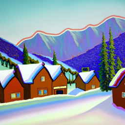
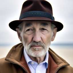

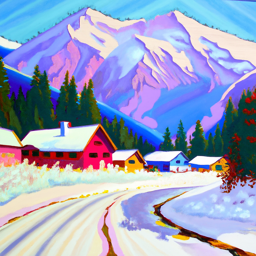
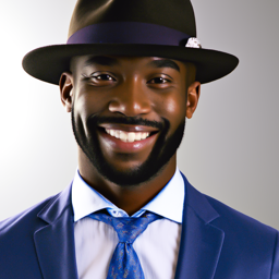

We can clearly see that a higher number of inference steps provides higher quality/detailed images.
Task 1: Forward Process
As diffusion models work by essentially denoising a noisy image, our first step is to actually blur an image. We’ll use the formula:
\[x_t = \sqrt{\bar\alpha_t} x_0 + \sqrt{1 - \bar\alpha_t} \epsilon \quad \text{where} \quad \epsilon \sim N(0, 1)\]To blur an image \(x_0\). The \(\bar\alpha_t\) can be adjusted based on a noise level variable that ranges from [0, 1000], with 0 being a clean image and 1000 being pure noise.
With the given test image below, we can try 3 different noise levels:


Task 2: Classical Denoising
Since the noise we added follows a guassian distribution, a simple way to denoise is to simply use a gaussian blur! Theoretically, this would average out much of the noise of the image, and although it’ll become blurry we can ignore some of the blur that was added. As we can see below, this works decently well for lower noises but at higher noises, we can really only make out the silhouette of the Campanile.


Task 3: One Step Denoising
A properly trained diffusion model can pretty accurately predict the noise that was added to any image, and thus by simply subtrating off the estimated noise, we should get a picture that is close to the original image. Using the same formula above, we can perform some algebra to get \(x_0\) from \(x_t\) and \(\epsilon\), our estimated noise.
\[x_0 = \frac{x_t - \sqrt{1 - \bar\alpha_t} \epsilon}{\sqrt{\bar\alpha_t}}\]Here are the results for each of the noise levels above:


Much better! But the image for the highest noise level is still quite blurry (and doesn’t resemble the campanile very well). Can we do better?
Task 3: Iterative Denoising
Instead of doing all the denoising one step, we can take iterative steps to slowly denoise an image bit by bit, to hopefully get a better result. The formula here:
\[x_{t'} = \frac{\sqrt{\bar\alpha_{t'}}\beta_t}{1 - \bar\alpha_t} x_0 + \frac{\sqrt{\alpha_t}(1 - \bar\alpha_{t'})}{1 - \bar\alpha_t} x_t + v_\sigma\]gives us \(x_t'\), which should be a slightly more denoised image compared to \(x_t\), until we eventually reach \(x_0\), the completely denoised image. Here’s the process on our most noisy image for t=750, showing a couple of steps in between.


Here are the 3 different technique’s results side by side.


We can see that the iteratively denoised campanile provided superior results: in both being less blurry and being more detailed (there are actual couds in the background!). The overall shape was also slightly better.
Task 4: Diffusion Model Sampling
Now, instead of passing in a blurred image, we can simply pass in what is essentially pure noise and see what the model comes up with.


Without any prompting or a base image to go with, the model just hallucinates some random images out. While we can make out some details in these images (street in the second image, scenery in the third and fourth?) this is mostly nonsense. They do definitely look feasible though, which is impressive.
Task 5: Classifier-Free Guidance
To improve on the quality and make the images look better, at the cost of “creativity”, we can use classifier free guidance. We’ll use our model to generate an unconditional prediction of the noise given an image, and a conditional prediction. Then, we can use the magical formula:
\[\epsilon = \epsilon_u + \gamma (\epsilon_c - \epsilon_u)\]To get our new noise which we will plug into the same equation above. We can clearly see here that at gamma=0, we just get the unconditional noise. At gamma=1, we get only conditional noise. Somehow, by setting gamma to some large number (we used 7), we get really good images! Here are the results:


As we can see, the images are now of much higher quality, although the variety has suffered a bit. Most of it has become either close-up shots of people or scenic imagery.
Task 6: Image to Image Translation
Now we can do something even more interesting - rather than passing in pure noise, what if we just took an image, add some noise, and then denoise it? This is really similar to what we did in task 3 except we’re now also using classifier-free guidance. We’ll try this at different noise levels, so that at lower noise levels we’ll get images that closely resemble the original image, and at higher noise levels we get almost completely different images instead.
Here are the original images;


And here are the denoised images, from most noise added to least noise added.


The Campanile managed to stay pretty much the same even with higher noise levels, but the same couldn’t be said for the other images. Perhaps it’s because there’s more buildings in the training set than the other two - almost immediately my cat became some bear hybrid and although Not-Batman pretty much stayed the same for the first couple of low-noise examples, it quickly became pictures of people again.
Task 7.1: Handdrawn and Web images
Although the image to image translation didn’t work too too well, what the model excels at doing is taking a nonrealistic image and making it into a more natural looking image. We’re going to use a couple of hand-drawn image and see how much noise it needs until it becomes a realistic picture, with an additional hyper-realistic image of a flower I found online as I’m curious how much noise needs to be added to that before it becomes something different.
original images:


Perhaps the most interesting things that happened here was how the crown and bread became ignored starting at i=10, becoming something completely different. Interestingly, the flower became 2 humans at i=7 but then returned as a near-identical flower at i=5, showing the randomness of diffusion models.
Task 7.2: Inpainting
Next we can attempt something interesting: Make a mask for an image, use the diffusion model to denoise the image, and after each iterative step we’ll leave everything inside the mask alone, but replace everything outside the mask with our original image. The end result will be that the denoising uses the surrounding pixels for denoising, but everything outside the mask is left alone.
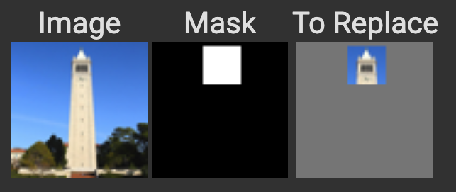

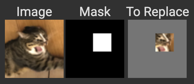

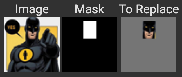

I intended the cat example to have made the facial expression different or replace it with some other animal, but it ended up looking like some eldritch horror. Truly traumatizing. The not-batman example was amazing though, providing a new face that could very much be a new villain.
Task 7.3: Text conditioned Image-to-Image Translation
Since we also have some text prompt embeddings loaded in, we can redo our timage to image translation but add some text for the diffusion model to work with. Again, we can use different noise levels for varying levels of editing.


Task 8: Visual Anagrams
An even cooler way we can use the diffusion model is to make optical illusions. First, we take two prompts and get noise estimates for each. We then apply one normally and apply the other to a flipped version of the image instead. The result is that we get an image that looks like the original prompt when looked at normally, and something completely different otherwise.


Task 9: Hybrid
Lastly, we can combine what we did in the earlier projects and make hybrid images. By using a low pass filter and a high pass filter, we can create hybrid images that will look different when viewed from afar vs viewed from nearby.


Trying different combinations of prompts together, it seems like similar prompts gave much much better results than others. The prompts used above all had similar mediums - oil paintings, lithographs, etc. - which made the end result more realistic.
Part B: Training our own Model!
All of the above depended on a great diffusion model that HuggingFace created, now, let’s make our own simple diffusion model. We can use the DDPM paper to implement a denoiser, providing the model architecture:
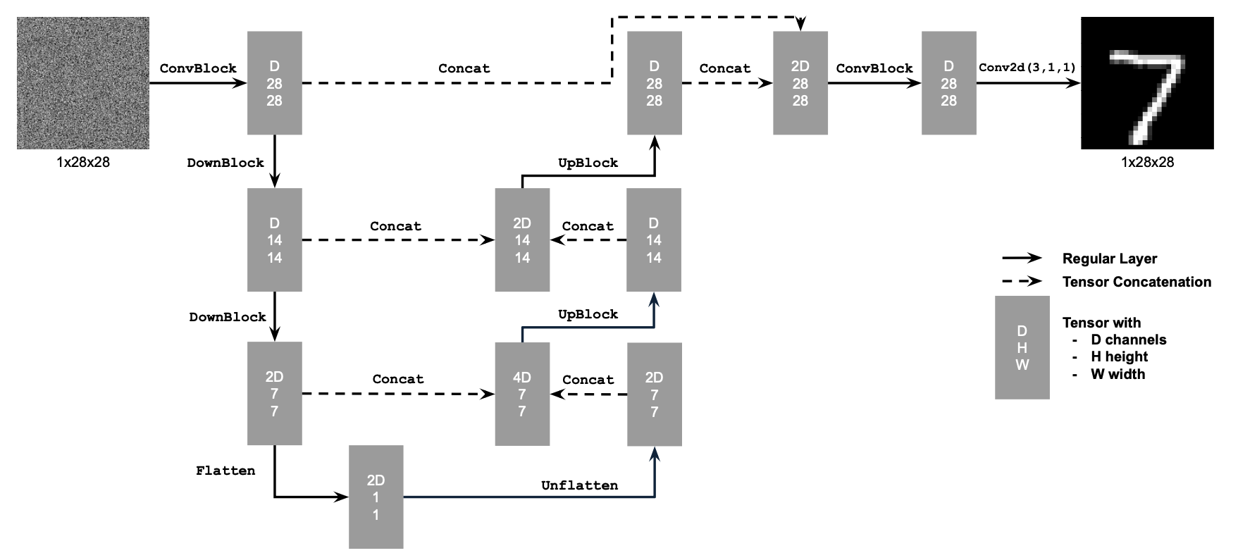
We need to feed in some noisy images for the model to predict the noise.
\[z = x + \sigma \epsilon,\quad \text{where }\epsilon \sim N(0, I). \tag{B.2}\]We can then optimize over L2 loss.
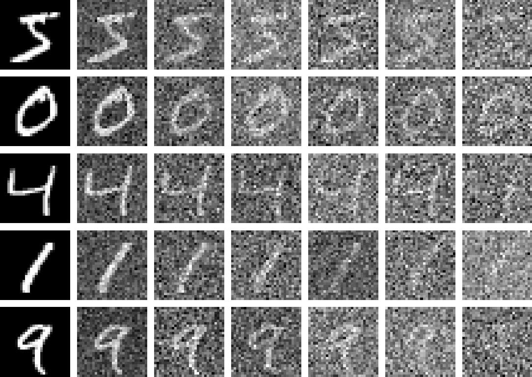
Here’s an example of digits being noised at different levels
Task 1: Training
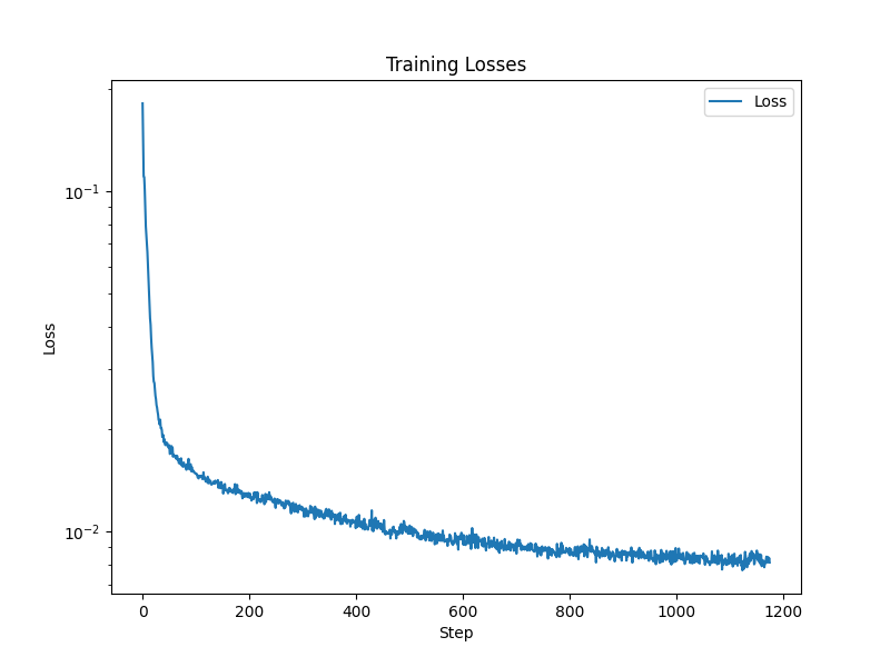
By noising a bunch of images with sigma=0.5 from the MNIST dataset and performing regression, we can train our model. Here’s the training loss curve over 5 epochs, with 256 batch size.
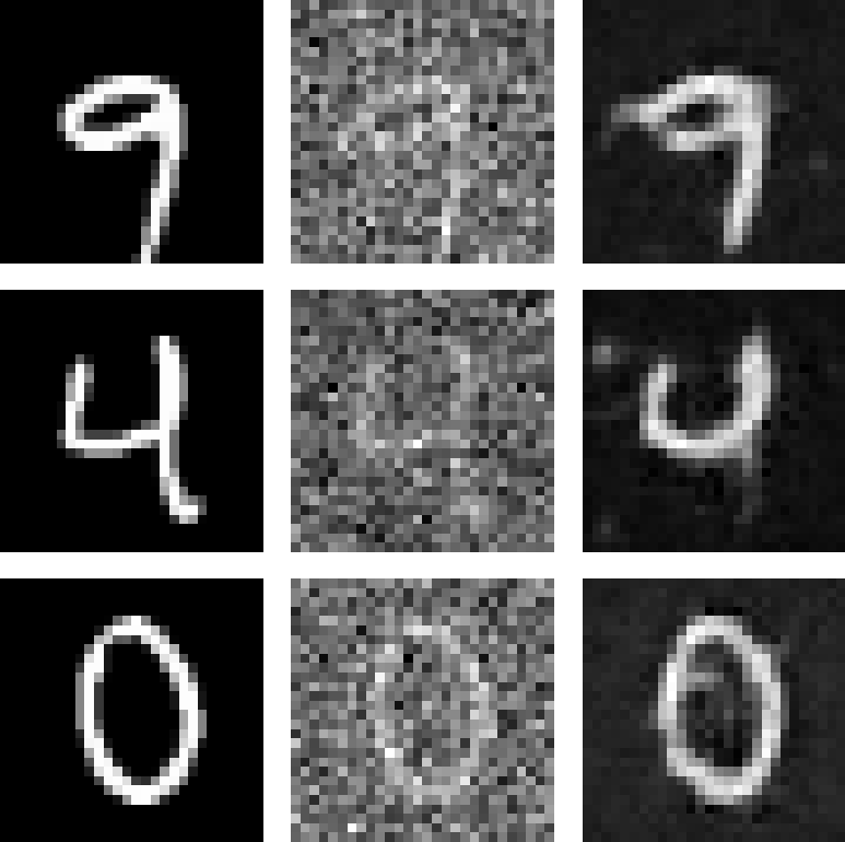
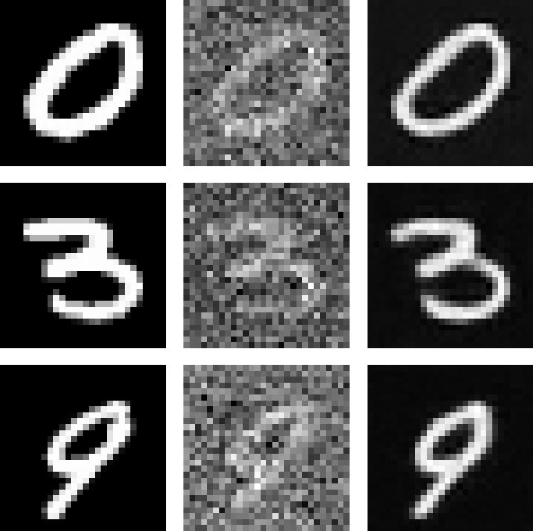
Now, our model is great at denoising mnist images with sigma=0.5! Here are some examples, for our model when we only trained for 1 epoch vs 5 epochs. We can see a clear improvement as we train for longer.
We can also test to see if it’s able to deal with other noise levels. Below, we take one MNIST image and run it through 6 different levels of sigma, then use our model to denoise.

As we can see, the model is decent at dealing with lower sigma values but falls short at higher values.
Task 2: Time Conditioning
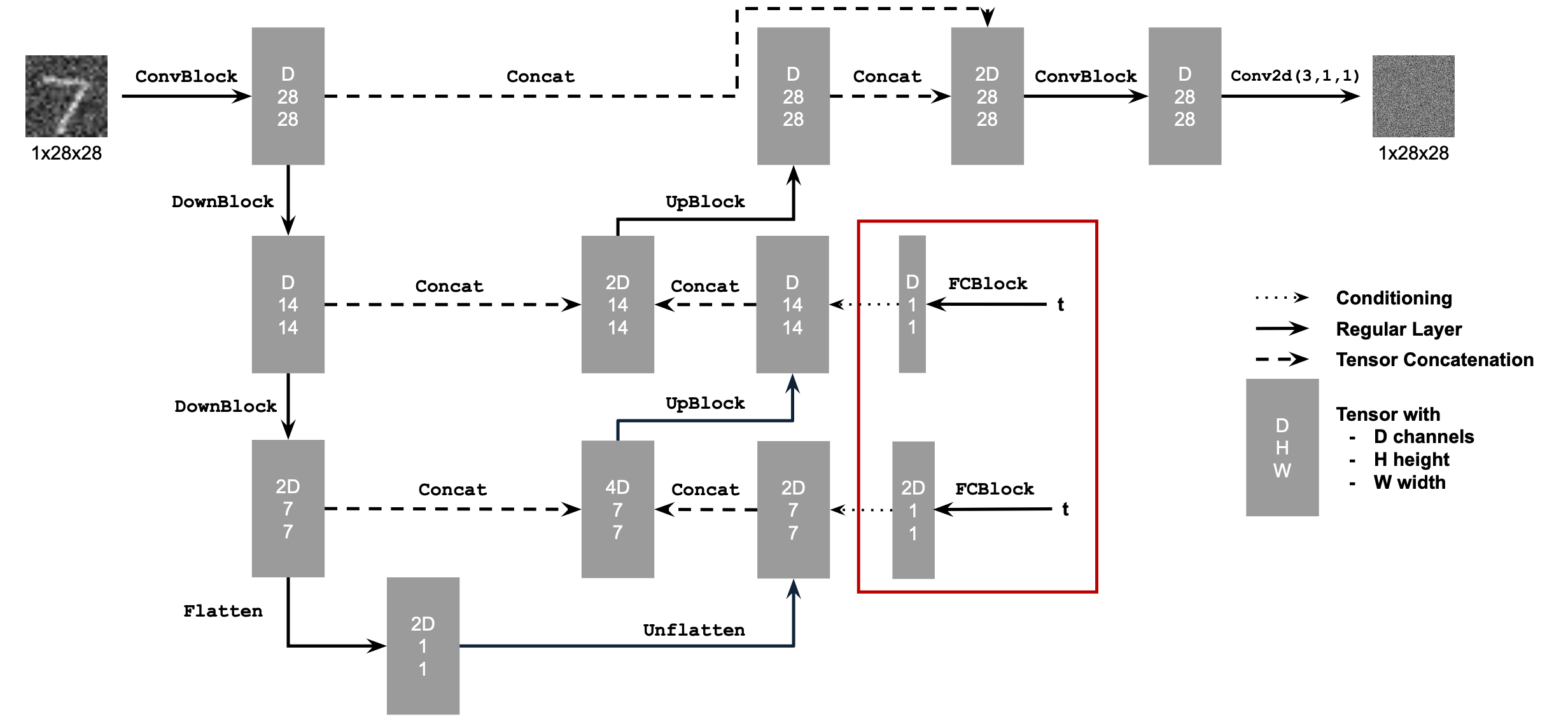
To actually train our model, we’ll need to add time conditioning. We’ll modify our architecture to add two FCBlocks that allow our model to be conditioned based on t. Architecture and training pseudocode below:

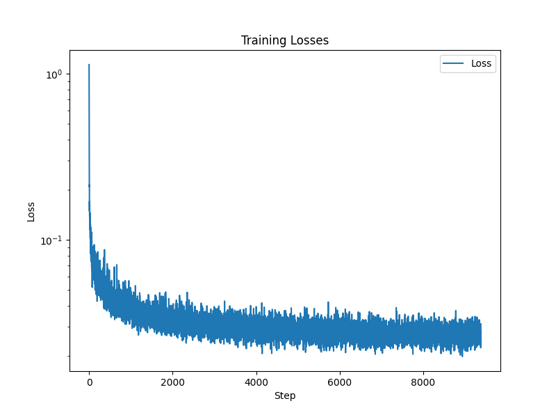
We’ll train with a batch size of 128 for 20 epochs using an exponential learning rate and the Adam optimizer. Here’s the training curve:
Now, we can sample form the Unet by passing in some pure noise and see what it comes up with. The algorithm for sampling is showed below, along with the results for 40 different tries at epoch 5 and at epoch 20.

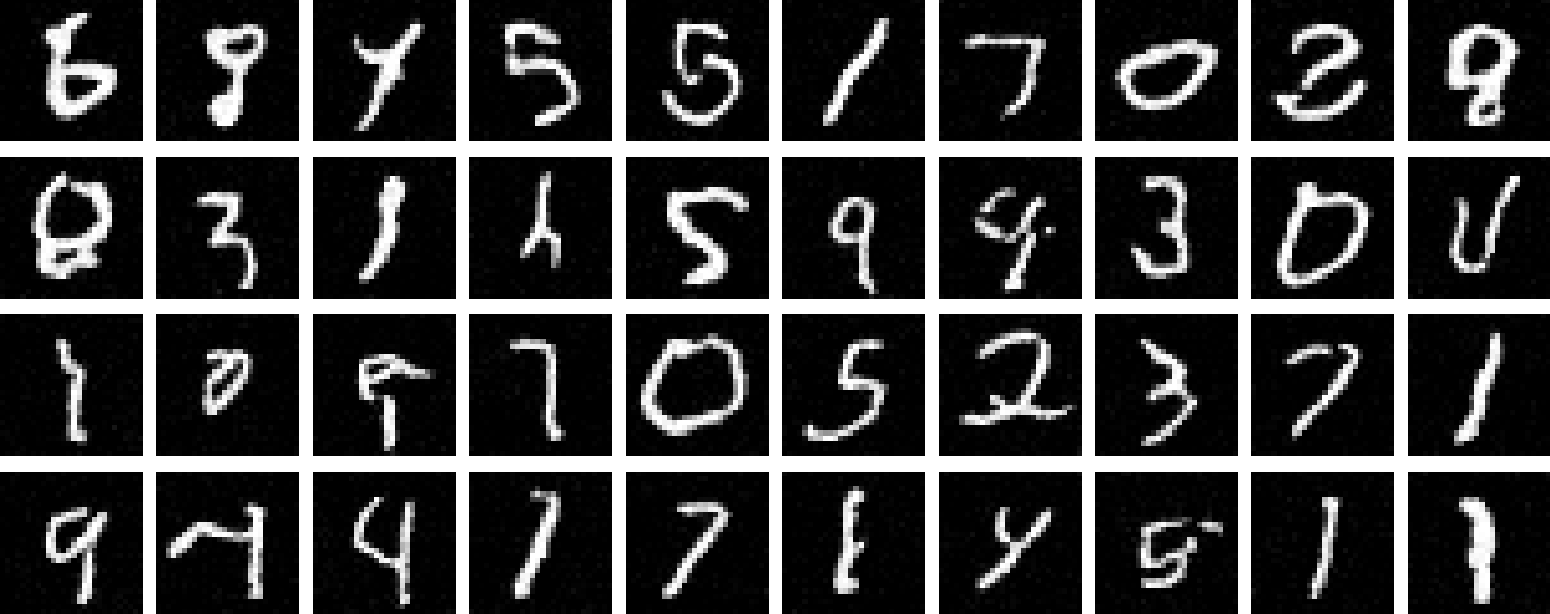
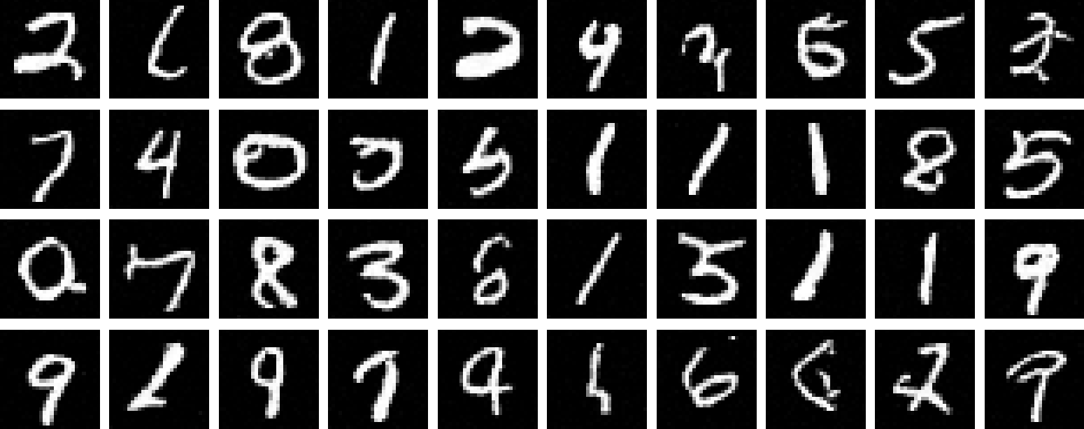
We can see that at epoch 20, our digits are much much better - there’s way fewer artifacts and lots of pretty well drawn numbers. It’s still not perfect though, and there are many nonsense digits. Can we do better?
Task 3: Class Conditioning
In addition to time conditioning, we can add 2 more FCBlocks to take in a class - the digit we want to create. We’d want to one-hot encode the digit first and pass in an array of size 10, one slot for each digit, and set the array to 1 at the index for the digit we want to generate. While training, we’ll also take a 10% chance to drop the entire array - so that it’s all 0s - so that the UNet can still perform unconditioned sampling. We’ll then use the same technique above with CFG and denoise using
\[\epsilon = \epsilon_u + \gamma (\epsilon_c - \epsilon_u)\]with a gamma of 5, to get our digit.
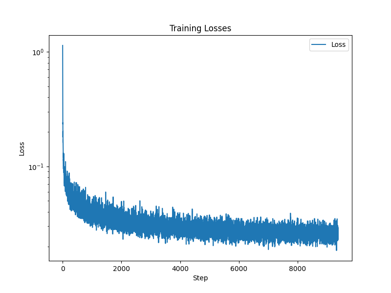
Here’s the training curve over 20 epochs:
And the results, for epoch 5 and 20, where we try each digit 4 times:
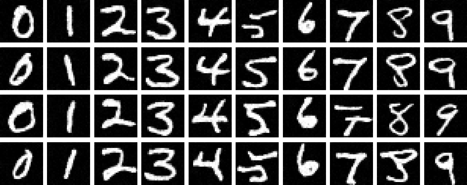
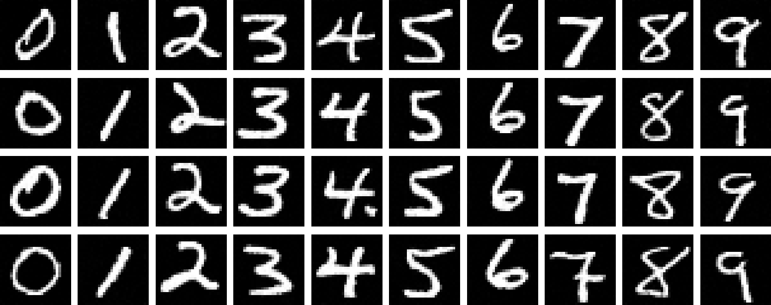
The accuracy at epoch=20 was pretty amazing - each digit is clearly visible and although there are a few artifacts, even their thicknesses were pretty uniform.
Conclusion
Overall, this project was a blast. It’s always super satisfying to understand something after being amazed by it for so long. Dall-E has been something I’ve been playing with since Freshman year and I’ve always wondered how it works, but never bothered to look deeply into it. This project gave a great introduction and idea of how things work under the hood, and it’s exciting to see what generative models will be able to achieve in the years to come.