Part 1: 2D Neural Field

Before we use a Neural Radiance Field to represent a 3D space, we can use a NeRF on a 2D example. Essentially, we’ll make a model that takes in a pixel coordinate {u, v} and output a color {r, g, b} in 2D space. We’ll use one image and train our model on it, then sample every single coordinate possible to get the resulting image. Of course, there’s really no need to do this as the image itself gives you the RGB value provided the coordinate, but this serves as a warmup.

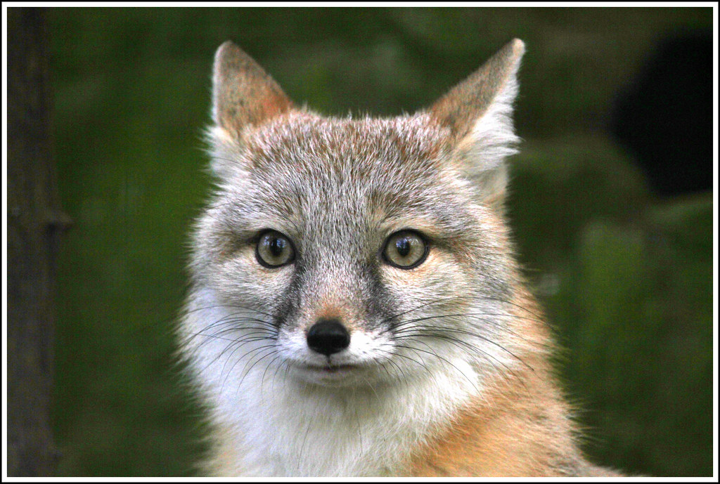
We’ll use the following architecture and try it the following two images.

Provided Image

Model Architecture

Custom Image

The PE refers to a Sinusoidal Encoding, applying sin and cos functions to the input coordinates to expand its dimensionality. Here, we use an L of 10, so we’ll expand our input from 2D (u, v) to 42.

\[PE(x) = \{x, \sin(2^0 \pi x), \cos(2^0 \pi x), \sin(2^1 \pi x), \cos(2^1 \pi x), \ldots, \sin(2^{L-1} \pi x), \cos(2^{L-1} \pi x)\}\]

Using a simple dataloader (that just randomly gets coordinates and provides the corresponding pixel color), the class architecture and running on the Adam Optimizer with a 1e-2 learning rate, MSE Loss, and 10k batch size for 2000 iterations, we get the results below for the provided fox image, along with the PSNR curve:

Fox over iterations ([1, 50, 100, 600, 1000, 2000])

PSNR over iterations

I also tried running some hyperparameter training on the provided image. Here’s the result of decreasing the number of layers from 4 to 3, and decreasing L from 10 to 6.

Fox over iterations ([1, 50, 100, 600, 1000, 2000]), small model

PSNR over iterations, small model

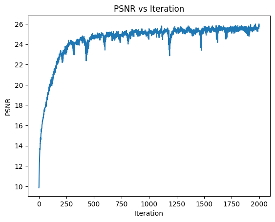
Surprisingly the results were still very good, which perhaps just shows how the task isn’t very complex and can be handled with a less sophisticated model.

Then, let’s try increasing the layers from 4 to 5, and L from 10 to 12 to make a big model.

Fox over iterations ([1, 50, 100, 600, 1000, 2000]), large model

PSNR over iterations, large model

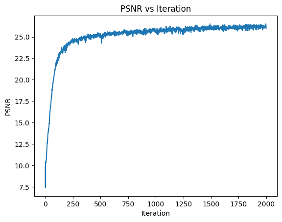
Tragedy. Interestingly we achieve a higher PSNR but the model clearly overfits.

Let’s now try using the smaller model, which we found to be effective, on the picture of my cat:

Cat over iterations ([1, 50, 100, 600, 1000, 2000]), small model

Cat over iterations, small model

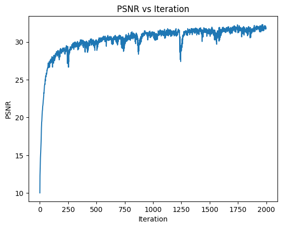
Surprisingy the smaller model is quite successful.

Part 2: 3D Neural Field

Part 2.1: Functions

Onto the real deal! As explained in class. We’ll get a bunch of images of a lego bulldozer from different angles, the camera coordinates, and other information (camera-to-world transformation matrices), train a powerful NeRF model on the information, and try to render the image from novel views given our information using some validation and test camera information that was provided.

First, we’ll implement three algorithms needed to train and sample: Camera to World Conversion, Pixel to Camera Coordinate Conversion, and Pixel to Ray conversion. All of these are taken from the course website and implement in pytorch.

$$ \begin{align} \begin{bmatrix} x_c \\ y_c \\ z_c \\ 1 \end{bmatrix} = \begin{bmatrix} \mathbf{R}_{3\times3} & \mathbf{t} \\ \mathbf{0}_{1\times3} & 1 \end{bmatrix} \begin{bmatrix} x_w \\ y_w \\ z_w \\ 1 \end{bmatrix} \end{align} $$

Camera to World Coordinate Conversion

$$ \begin{align} \mathbf{K} = \begin{bmatrix} f_x & 0 & o_x \\ 0 & f_y & o_y \\ 0 & 0 & 1 \end{bmatrix} \end{align} $$ $$ \begin{align} s \begin{bmatrix} u \\ v \\ 1 \end{bmatrix} = \mathbf{K} \begin{bmatrix} x_c \\ y_c \\ z_c \end{bmatrix} \end{align} $$

Pixel to Camera Coordinate Conversion

$$ \begin{align} \mathbf{r}_o = -\mathbf{R}_{3\times3}^{-1}\mathbf{t} \end{align} $$ $$ \begin{align} \mathbf{r}_d = \frac{\mathbf{X_w} - \mathbf{r}_o}{||\mathbf{X_w} - \mathbf{r}_o||_2} \end{align} $$

Pixel To Ray

To get the W2C matrix for extracting R and T in Pixel To Ray, I simply used the inverse of C2W that was passed in.

Part 2.2: DataLoader

Next, we’ll need to make a DataLoader that can be used to provide our model with information. The goal is for the dataloader to provide two sampling functions: sample_rays(num_rays) and sample_along_rays(rays_o, rays_d, perturb). As the DataLoader will only be loaded in once while sample_rays will be run thousands of times, I optimized the dataloader such that all possible rays and pixels are pre-computed, and sample_rays can then simply index into the vast number of rays and pixels as data.

The Dataset takes in the training images, an intrinsic matrix K, and each image’s camera2world matrix.

For each image, we’ll get every single possible coordinate and its corresponding pixel value (uv), and store it.
Shift the coordinates by 0.5, so that the ray points at the middle of the pixel rather than a corner.
Use the pixel_to_ray formula above to get a list of all ray origins and ray directions for all pixels.

Then, to sample we’ll just simply randomly select without replacement a list of indices from our list of all pixel values, and use the corresponding indices to get the uv, ray_o, and ray_d.

For the sample_along_rays function I followed the staff formula and set n_samples to 64, near=2, far=6, and t_width=0.02. We also introduce perturbations so that the points aren’t evenly spaced for each ray to prevent overfitting.

Part 2.3: Visualization

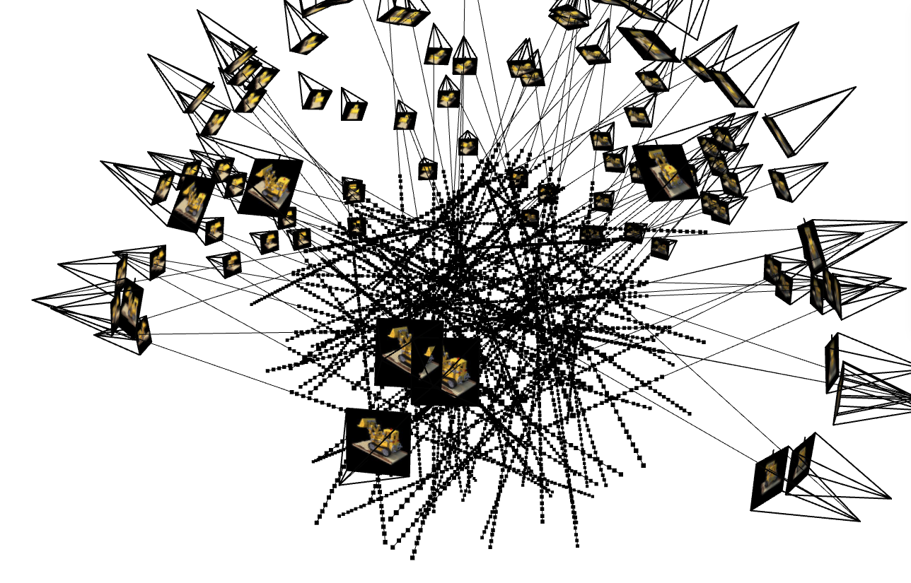
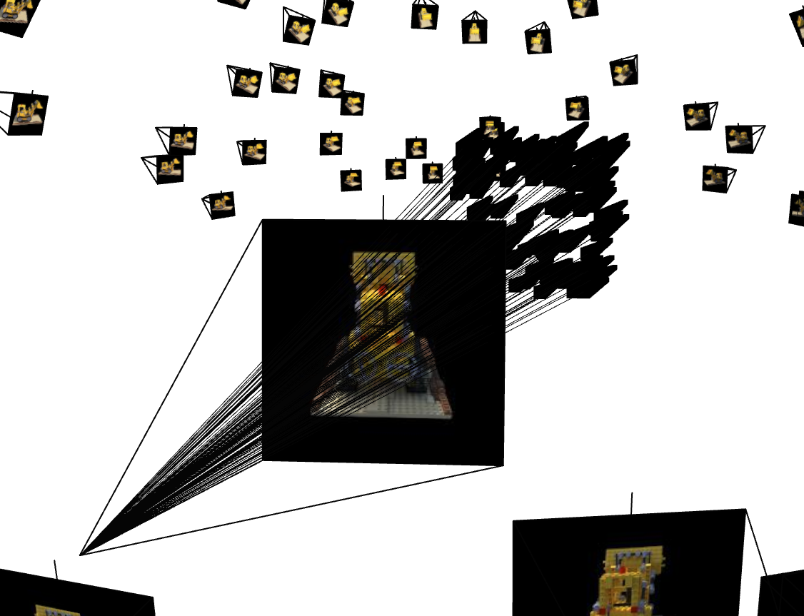
Plugging in the staff code to ensure my code thus far has been working well, we can see a visualization of 100 randomly selected rays amongst all our cameras, as well as the perturbations we introduced in sample_along_rays. During one training loop, we’ll use 10,000 rays instead. I also included 100 rays only for 1 image on the top right corner, provided by the staff visualization code.

100 rays with num_samples=64 and perturbations

100 rays with num_samples=64, top right of camera 1

Part 2.4: Neural Radiance Field

For the model, I used the staff provided architecture:

With Hyperparameters/parameters:

L_x=10, L_d=4, num_hidden=256
Adam optimizer, lr=8e-4
ExponentialLR scheduler, gamma=0.9999
5000 iterations (later increased to 30,000)
10k batch_size
64 num_samples in sample_along_rays, with t_width=2.0

Part 2.5: Volume Rendering

The model outputs a density and RGB. To actually get the final color of a pixel, we’ll need to combine the rgb/densities we collected from the model at each point using the staff formula, which I implemented using pytorch.:

$$ \begin{align} C(\mathbf{r})=\int_{t_n}^{t_f} T(t) \sigma(\mathbf{r}(t)) \mathbf{c}(\mathbf{r}(t), \mathbf{d}) d t, \text { where } T(t)=\exp \left(-\int_{t_n}^t \sigma(\mathbf{r}(s)) d s\right) \end{align} $$

Real formula

$$ \begin{align} \hat{C}(\mathbf{r})=\sum_{i=1}^N T_i\left(1-\exp \left(-\sigma_i \delta_i\right)\right) \mathbf{c}_i, \text { where } T_i=\exp \left(-\sum_{j=1}^{i-1} \sigma_j \delta_j\right) \end{align} $$

Our discrete approximation

Results:

Here’s many samples from various iterations for validation camera 1, with the real image on the left.

Samples from model (expected | iter=100, 200, 400, 1000, 2000, 5000)

Here are the corresponding PSNR curve comparing with 6 images from the validation set (which we’ll check every 100 iterations). I also included the corresponding training psnr (which is collected every iteration).

training and validation PNSR

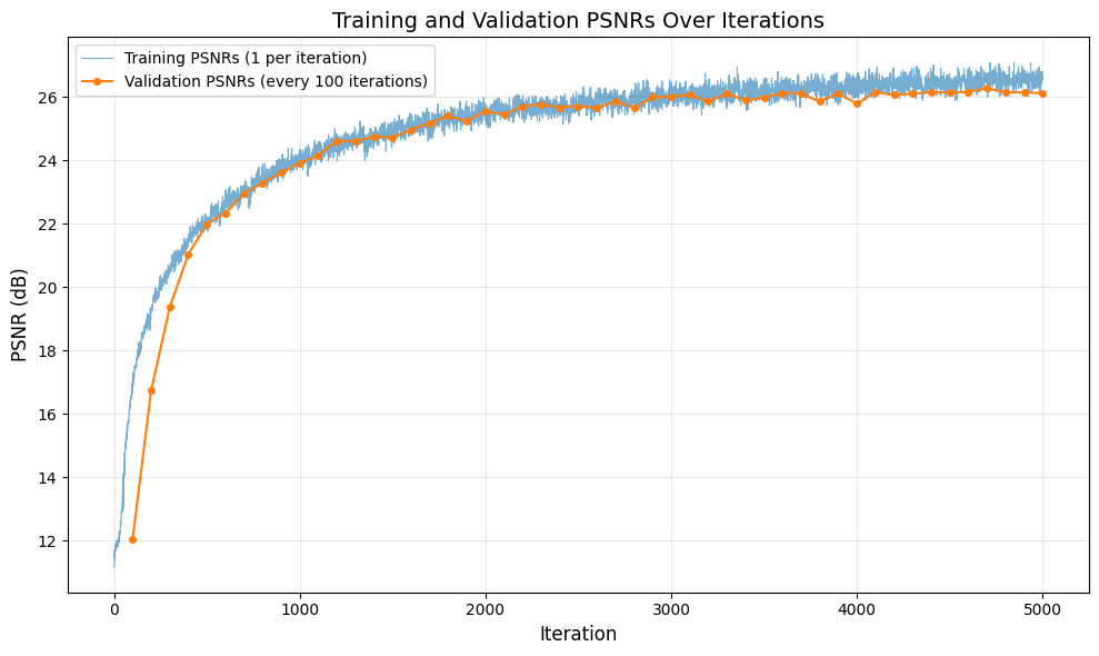
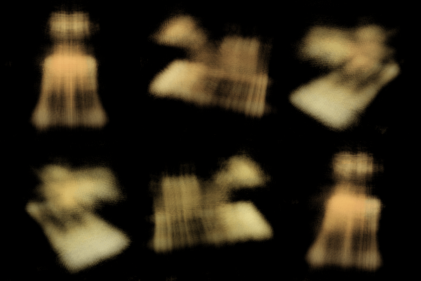
We can clearly see that it plateaus around 5000 iterations. Let’s now sample from the test cameras at different iterations and see how the model evolves, by creating a gif for all the camera angles provided in the test_c2ws:

If the gifs are not working, it’s probably because it didn’t loop. Reload the page or open the image in a new tab to view it clearly.

100 gradient steps

200 gradient steps

400 gradient steps

1000 gradient steps

2000 gradient steps

5000 gradient steps

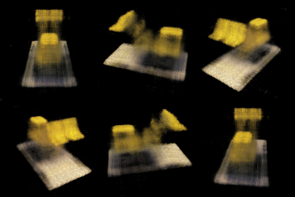
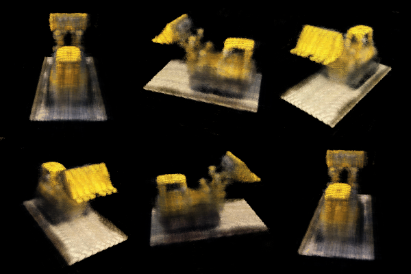
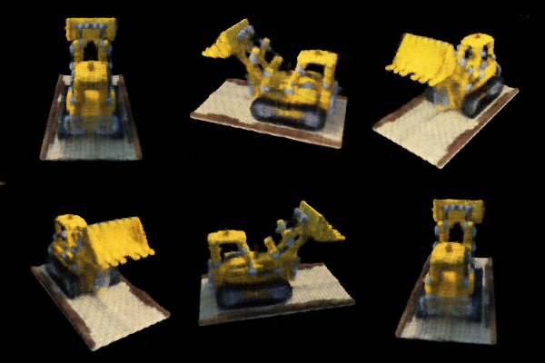
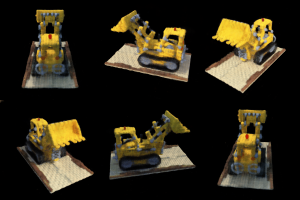
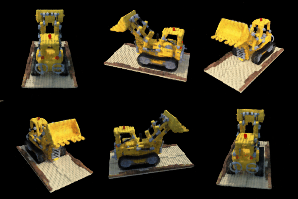
And just for fun, I decided to train for about 3 hours, up to 30000 iterations. Here are the results:

10000 gradient steps

15000 gradient steps

20000 gradient steps

30000 gradient steps

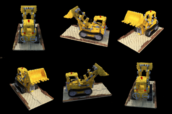
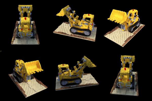
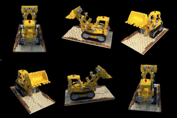
As we can see, the differences aren’t that significant. Although it’s pretty interesting it didn’t overfit and cause strange things to start happening.

Bell and Whistle

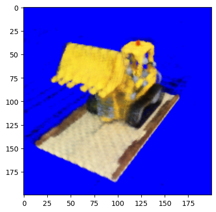
By simply modifying our volrend function, we can add background color. Basically, we want to render and return the background color in the case that our ray “hits” nothing, which currently gives us black. By examining our equation above, we can think of T as a weight for the color provided by the model. By adding a (1-T) * bg_color term, we can inject background color:

background color injected

Conclusions

Overall this was by far the hardest project in the semester. The provided staff code, explanations, and formulas were extremely useful in the implementation, and the sense of triumph as I got the first gif is indescribable.